After hours of work, you have finally finished compiling the large data set.
But now that you’re looking at the worksheet, it does not look appealing.
It’s pretty hard to keep track of each row or make something out of the vast dataset.
So you feel the need to make it visually appealing and more readable by highlighting alternate rows.
Luckily, you can highlight every other row (or column) in Excel.
This post will guide you through different ways to highlight alternate rows (and columns).
After going through the entire post, you’ll be able to shade every other row in Excel quickly.
So read the post till the end.
How To Highlight Every Other Row In Excel
Knowing how to highlight alternate rows is an essential skill in Excel.
Highlighting alternate rows in Excel makes the data more visually appealing and readable. Any person can quickly find the required data and keep track of a long row if the alternate rows have different colors.
It’s essential not to use any dark shade of color while highlighting. Though it might look good on screen, a printed copy will be hard to read.
There are two ways to highlight every other row (or column) in Excel: using conditional formatting and Excel tables. Both methods have their advantages and disadvantages.
I will go through both methods now, and you can pick one based on your preferences.
Related guide: how to Make a Histogram in Excel.
Follow the methods below to shade every other row in Excel:
1. Use tables
Using Excel tables is the fastest way to highlight alternate rows. In this method, you would format the data as a table.
Many styles are available for tables in Excel. These table styles have default color banding as their style configuration. So formatting the data as a table automatically shades every other row in Excel.
There are also some added advantages of using Excel tables.
When you add more rows, the alternate row highlighting is automatically applied to the new rows. So you don’t have to highlight the new rows manually. The same goes for row deletion.
Moreover, Excel tables display total and header rows. Filter drop-down lists are also available, which can help find the required data quickly.
Also, check out our separate post on Microsoft Excel Freezing or Slow.
Here are the steps to highlight every other row in a table:
- Open the worksheet.
- Select the cells of data.
- Switch to the Home tab from the top.
- Click on “Format as Table” under the Styles group. You will see an extensive list of table styles.
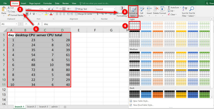
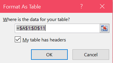
- Select a table style from the list. It’s better to choose from the “light” styles for better print output. You will see a new Format As Table window.
- Check “My table has headers” if your data has a header row.
- Click OK.
- Select any cell in the table.
- Go to the “Design” tab from the top.
- Ensure “Banded Rows” is checked in the “Table Style Options” group. If you want to highlight every other column instead of rows, uncheck “Banded Rows” and check “Banded Columns.” You can also hide Filter Buttons if you wish.
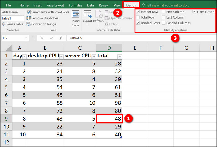
You should find the data now more visually appealing with every other row highlighted.
But what if you want to shade alternate rows in Excel without a table? Maybe you don’t want the Excel table functionality on your data.
In such a case, you have two options: You can follow the second method (conditional formatting) or convert the table back to a Data Range.
Let’s discuss how to convert the table to a Data Range, and then we will move to the following method. To convert the table back to a Data Range, you must perform additional steps after the above steps.
Here’s a complete guide on how to Highlight Duplicates In Excel.
The additional steps are:
Click on any cell in the table, then switch to the Design tab from the top. Select “Convert to Range” in the Tools group. Click Yes to confirm, and the whole table will be converted back to a Data Range. 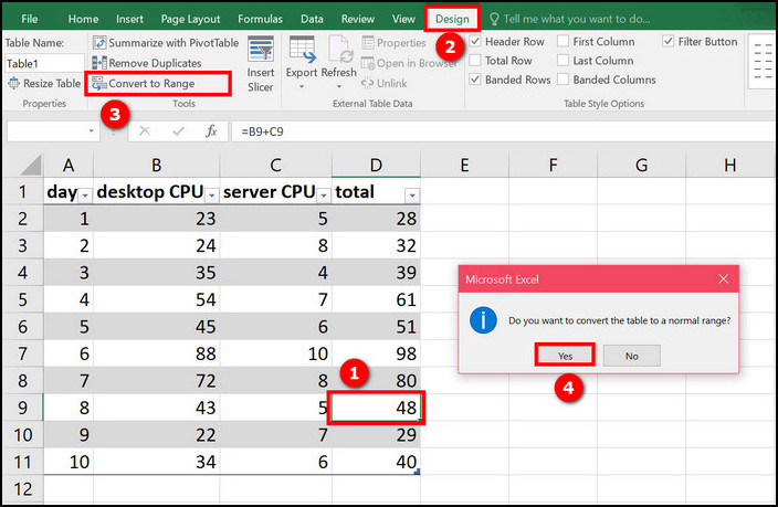
Alternatively, right-click on the table to bring up the context menu. Go to Table > Convert to Range.
Converting the table back to Data Range will keep the table styling (which includes the row highlighting) but remove the Excel table functionality.
More importantly, new rows will not get highlighted if you convert the table to a Data Range. In that case, you can use Format Painter to copy alternate row highlighting to the new rows.
To use Format Painter, select the rows from which you want to copy the style. Then go to the Home tab and click the “Format Painter” button on the top ribbon. Now drag to select the new rows where you want to apply the alternate row highlighting.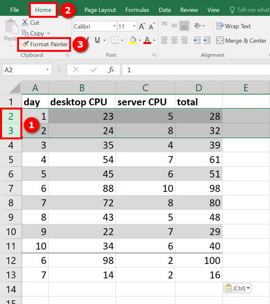
After selecting the rows, release the mouse, and the highlighting will be applied instantly. 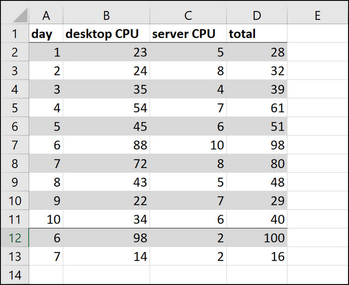
Obviously, if you regularly add new rows to your worksheet, using Format Painter to highlight the rows manually will be a pain.
So, using Excel tables to highlight rows and then converting the table back to Data Range should be done only when working with a fixed dataset.
If you are to add new rows, you should follow any of the two routes: keep using Excel tables (i.e., don’t convert the tables to Data Range) or use the following method (conditional formatting).
Check our epic guide on how to Freeze Panes In Excel Easily.
2. Use conditional formatting
Conditional formatting is a powerful tool in Excel. It uses formulas and conditioning to format a range of cells.
But don’t worry if you fear Excel formulas. I’ll provide the required formula here (a pretty easy one) and also explain how it works.
The benefit of using conditional formatting to highlight every other row is that new rows will be highlighted automatically.
Here is the procedure:
- Open the worksheet containing the data.
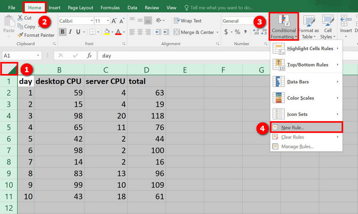
- Select the cells you want to highlight. If you want to highlight new rows automatically, click on the Select All button on the top-left of cells.
- Switch to the Home tab.
- Click on the Conditional Formatting button on the top ribbon. You will see a drop-down list.
- Select “New Rule” from the drop-down list. The New Formatting Rule window will appear. Alternatively, use the keyboard shortcut: Alt+O+D.
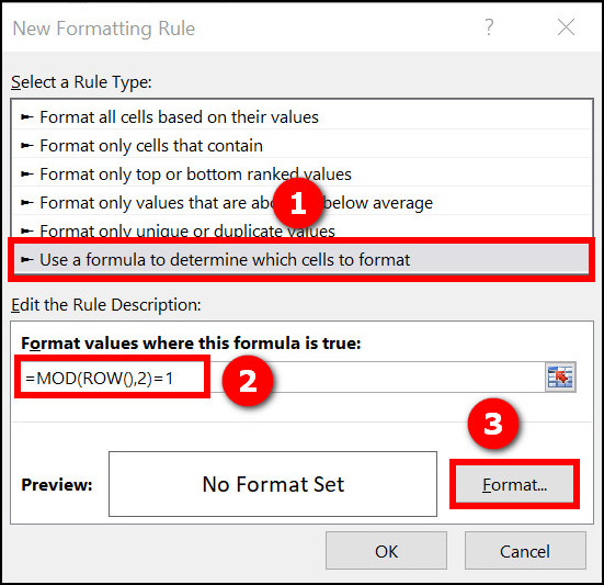
- Click on the “Select a Rule Type” drop-down and choose the “Use a formula to determine which cells to format” option. If you’re on a Mac, Select “Classic” as the style.
- Paste the following formula to the “Format values where this formula is true” box (without quotes): “=MOD(ROW(),2)=1“.
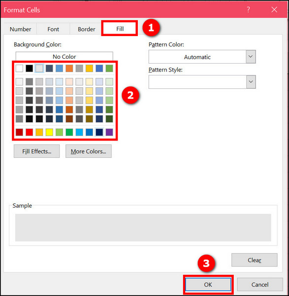
- Click on the Format button. A new window will appear.
- Select Fill from the top.
- Choose a color. You can preview how the output will be in the Preview box.
- Click OK. The Format window will close.
- Click OK on the “New Formatting Rule” window to apply the formatting.
Now you should see every other row highlighted in your worksheet. 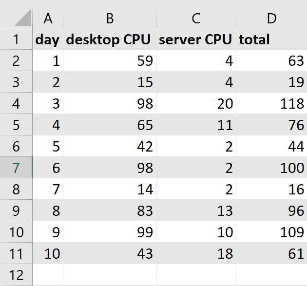
Let’s dive deep into the formula and see how it works. Then you will be able to modify the formula for more advanced highlighting (making a tri-band or highlighting every three dows, for example).
ROW() returns the row number. So calling ROW() on cell A2 will return 2, whereas calling it on cell A3 will return 3.
MOD(x,y) divides x by y and returns the remainder. So MOD(2,2) will return 0 (since there is no remainder when 2 is divided by 2). MOD(3,2) will return 1 since the remainder is 1 when 3 is divided by 2. MOD(4,2) will return 0 since the remainder is 0 when 2 divides 4.
Have you noticed the pattern here? In the formula MOD(x,2), when x is an even number, the result is 0. When x is an odd number, the result is 1.
We can use this realization to determine whether a row is even or odd. Then we can apply the highlighting to every even or odd row (which will highlight alternate rows).
Therefore, if you use the formula “=MOD(ROW(),2)=0” it will be applicable for every even row. The formula “=MOD(ROW(),2)=1” will be applicable for every odd row.
Once the formula determines either the even or the odd rows, Excel applies the selected style to the rows. That’s how the conditional formatting method works.
Now, if you want to highlight alternate rows in groups of three (that is, the formatting will cycle every three rows), you can use the following formulas:
“=MOD(ROW(),3)=0” to highlight every third row and “=MOD(ROW(),3)=2” to highlight every second row. So you need to apply two rules instead of one. The result would look like this: 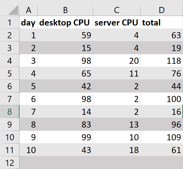
Select any cell with the rule if you want to edit the conditional formatting rule. Then go to Home > Conditional Formatting > Manage Rules and click on Edit Rule.
You can use Format Painter to apply conditional formatting to different cells. It’s helpful if you have already applied the formatting to some columns and now want to extend it to more columns.
To copy conditional formatting rules to new cells, select any cell where the rule is applied. Then go to Home > Format Painter and drag the mouse over the cells to which you want to apply the formatting.
Using COLUMN() instead of ROW(), you can highlight alternate columns using conditional formatting.
Final Thoughts
Highlighting every other row in Excel makes the data more readable as it becomes easier to read data from a long row.
You can either use Excel tables or conditional formatting to highlight alternate rows (or columns) in Excel. If you don’t like tables, you can convert them back to Data Range after highlighting (though it has some drawbacks).
I prefer the conditional formatting method because of its flexibility. But if the Excel formula is not your cup of tea, using the table method is straightforward.