Have you been trying to lock a certain row or column in Microsoft Excel before viewing a huge amount of data but cannot figure out how to do it?
If the answer to this question is yes, then this guide is meant for you.
Microsoft Excel allows you to freeze any panes on a spreadsheet and this feature might be hard to find among all the other important and useful facilities that Excel provides. The way of freezing panes is clearly discussed in this guide.
So keep reading if you want to know how to effortlessly freeze panes in Microsoft Excel.
What happens when you freeze panes in Excel?
Excel users have to work with a huge amount of data on a single spreadsheet. To do this, the app has a lot of great features that make room for a lot of versatility for users.
As a spreadsheet app, Microsoft Excel has sorts of spreadsheet tools and more.
Freezing panes is one of the neat features available in Excel and it comes in handy in many situations, such as when you need to keep the top header rows locked to make viewing your data more relevant, or if you want to lock a certain number of columns and scroll through the rest to compare. 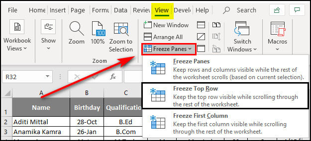
This feature has many types of applications depending what you are using it for.
Microsoft Excel provides a few options when it comes to freezing panes. These options and how they work are described in easy words on the next section of this guide.
Go through the following section in order to know about different freeze pane options and how to use them according to your preference.
How do you freeze panes in Microsoft Excel?
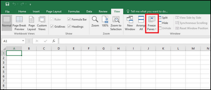
The freeze panes feature in Excel can be a little confusing to understand at first but it is actually a very simple feature that can come in handy during your spreadsheet tasks. The tool is within the View tab of Microsoft Excel app.
Freeze panes options allow you to lock any number of rows or columns on Excel but it also has a limitation. It only allows locking rows from the top and/or columns from the left.
You cannot freeze specific row or column in the middle of the spreadsheet.
Depending on your purpose, you may want to freeze only the top row or the first column, certain number of rows or columns, or you may want to freeze a number of rows and columns together. You can find out the ways of doing it easily explained here.
Follow these steps to know how to freeze pains in Excel:
1. Freeze the topmost row
The top row on spreadsheets is usually the header which contains the labels about the data that exist on the following rows. If you scroll through the data without locking the header, then you won’t be able to see it when you scroll down further into the spreadsheet.
So, in order to keep the header on screen, you will have to freeze the first row using freeze panes feature in Excel. The process of doing it is actually very simple.
Here’s how you can freeze only the top row in Excel spreadsheet:
- Use Excel to open your spreadsheet.
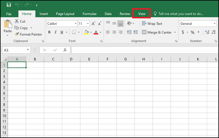
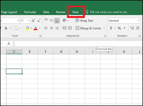
- Select View tab in Microsoft Excel when you open your spreadsheet.
- Expand Freeze Panes menu.
- Click on Freeze Top Row.
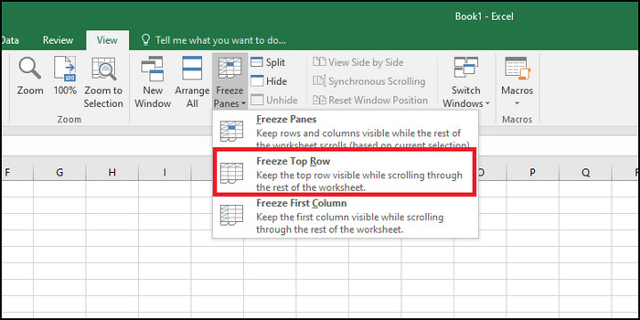
When you have followed these steps and frozen the top row, it will be locked and Excel will make its separator line bolder to indicate that it is frozen. Then you can scroll through the data freely without having the row move away from the screen.
2. Freeze the first column
If you want to lock the data on just the first column on Microsoft Excel to freely scroll the rest of your spreadsheet, you can also do it very easily using freeze panes.
This is how to freeze just the first column by using Excel:
- Run Microsoft Excel and open your spreadsheet document.
- Select View tab in Excel after opening your spreadsheet.
- Expand Freeze Panes options.
- Click on Freeze First Column.
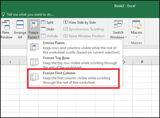
This will then lock the first column in Excel and if you scroll to the right, it will remain in place on your screen even when the rest of the columns move away. It will be indicated by bold separator line.
3. Freeze certain number of rows
You can also freeze any certain number of rows you want in Excel using freeze panes. The limitation is that the frozen rows will have to start from the top of the spreadsheet file.
Go through these steps to freeze multiple rows at once in Excel:
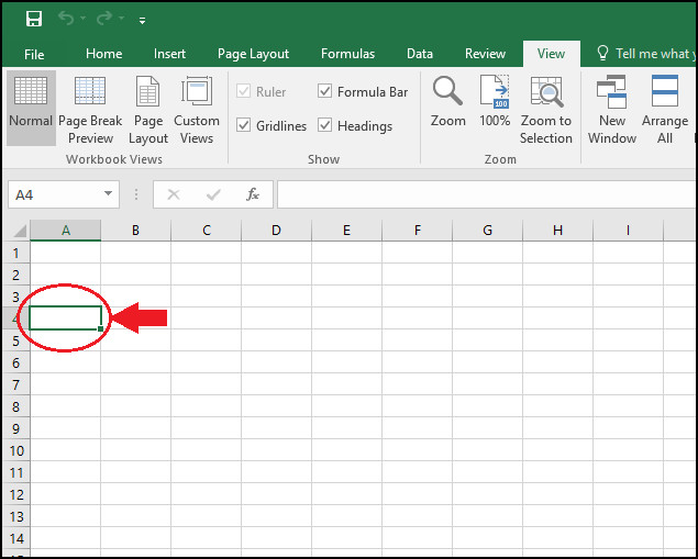
- Open your spreadsheet using Excel.
- Click on the cell on first column right under the last row you want to freeze from top. For example, if you want to freeze first 3 rows, then you have to click on cell A4.
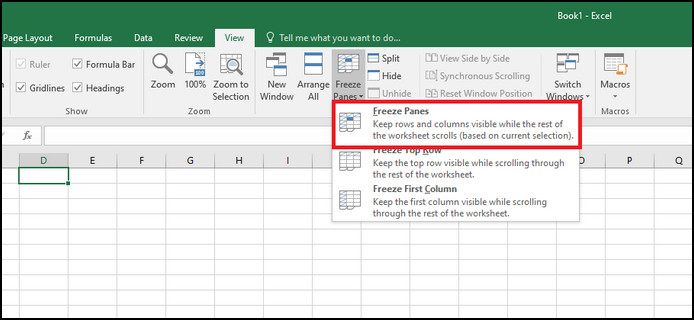
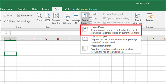
- Go to Freeze Panes menu.
- Select Freeze Panes.
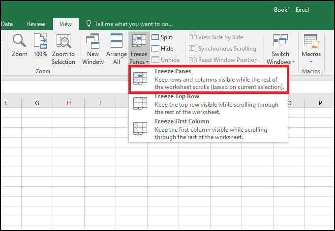
The rows you have frozen will then be grouped together on your screen and stay locked while you scroll until you unfreeze them again.
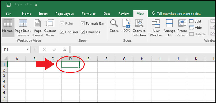
4. Freeze specific number of columns
Besides multiple rows, you can also freeze specific number of columns at a time using freeze panes feature in Excel.
Follow this process to freeze multiple columns at once In Excel:
- Run Microsoft Excel and open your spreadsheet.
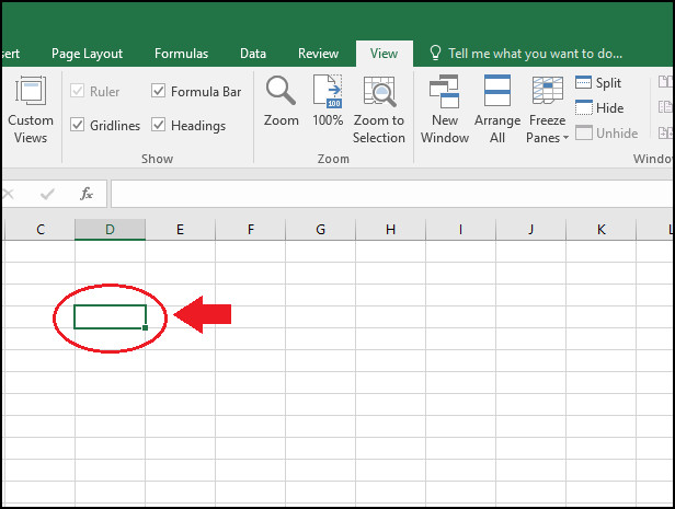
- Click on the cell on first row that is to the right of last column you want to freeze. For example, if you want to freeze first 3 columns, then you have to click on cell D1.
- Go to Freeze Panes menu.
- Select Freeze Panes.
After you have done this, the specific number of columns you want frozen will then be locked in place. They won’t move away from the screen now if you scroll from left to right.
5. Freeze rows and columns together
Freezing columns or rows is very useful but what about doing it together? You can also lock any number of columns and rows together at the same time in Excel by using Freeze Panes.
Take these steps to freeze one or multiple rows and columns together in Excel:
- Run Excel and open your spreadsheet file.
- Click on the cell under the last row AND on the right of the last column you want freeze. For example, if you want to freeze first 3 rows and columns, then you have to click on cell D4.
- Open Freeze Panes menu.
- Click on Freeze Panes.
When you have gone through these steps, the rows and columns you have locked will be separated by a bold line, indicating that they are now frozen. This is means that you can scroll in whichever direction you want and these rows and columns will always stay on your screen.
How to unfreeze panes in Excel?
By now you should know all the ways in which you can freeze panes but what about unfreezing them again?
It is actually just a simple process like the methods of freezing the rows and columns. The unfreezing option is available in Freeze Panes if you have already frozen any of the panes.
To unfreeze your rows or columns, follow these steps:
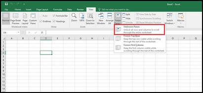
- Go to View tab after freezing your panes.
- Expand Freeze Panes.
- Select Unfreeze Panes.
Conclusion
Microsoft Excel provides with all the resourceful tools you need while working on a spreadsheet document. Freeze panes is one such tool that you can use to efficiently traverse your spreadsheet.
So, if you want to learn this effective feature and make it so that it is only a matter of few clicks for you, learn the processes in this guide.