Imagine this, you are working with a huge amount of data on a spreadsheet using Microsoft Excel and you notice that a few duplicate entries of the same data appear two or more times in the spreadsheet. What do you do then?
You clearly have to find out all the duplicates and remove them from the spreadsheet.
Obviously, you are not going to do this manually because Excel has the feature of highlighting and managing duplicate data on your spreadsheet all at once. This guide discusses this feature of highlighting the duplicates in detail.

So keep reading if you want to know how to highlight duplicate data in Excel and keep the unique values in columns.
Why happens when you highlight duplicates in Excel?
When working on a spreadsheet, you may come across many duplicate data entries that you may have to remove.
To do this, you have to first find out all the duplicate entries within the set of data.
This is where highlighting duplicates in MS Excel comes in. It is basically a spreadsheet formatting rule that you can use to pinpoint the same data existing twice or more times in your file. 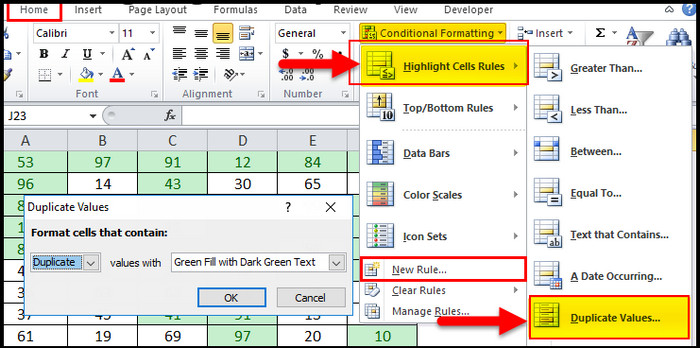
Highlighting duplicates can be done in several ways. There is a built-in rule for it but you can also make your own custom formatting rule to highlight data in multiple and/or specific columns.
The ways of doing this in Microsoft Excel are described in the next section of this guide. The processes are explained in detail but also in a simple way so that they are easy to understand.
So move on to the following section to find out how to highlight the duplicates in Microsoft Excel.
How to highlight duplicate data in Excel?
Highlighting the duplicates within your spreadsheet in Excel is simple task and it is also very resourceful. You can find and highlight duplicates values in one or more columns using the built-in duplicate highlighting rule or create a custom rule to highlight the duplicate rows.
The ways of highlighting the identical data present throughout the spreadsheet are shown in the following steps.
Go through these steps on how to highlight duplicates in Excel:
1. Highlight duplicate data in a single column
If you have the same data appearing in multiple cells in one column, then you can highlight those very easily. For this, you have to use Conditional Formatting rules. This rule highlights all the data that appears twice or more times in the column that you will selectt.
Here’s how to highlight duplicates in one column of Excel:
- Open your desired spreadsheet using Microsoft Excel.
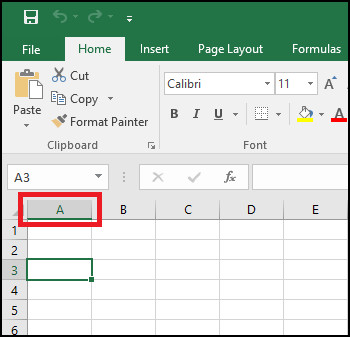
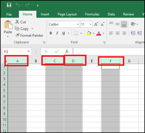
- Click on the top of the column you want to highlight duplicates from to select it.
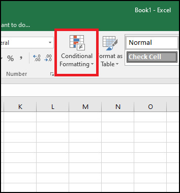
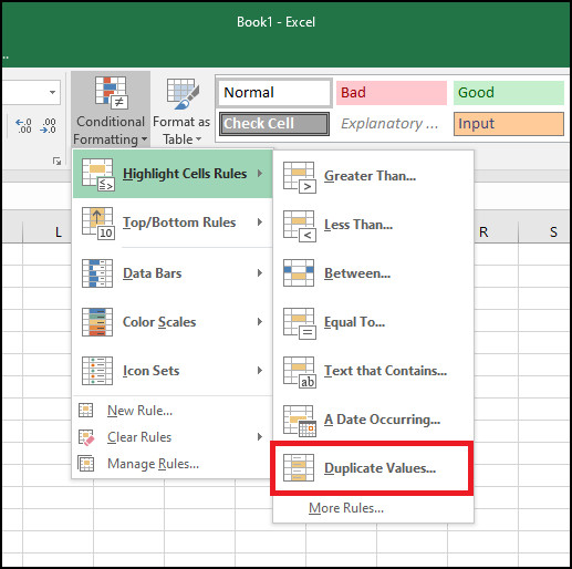
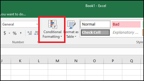
- Expand Conditional Formatting menu.
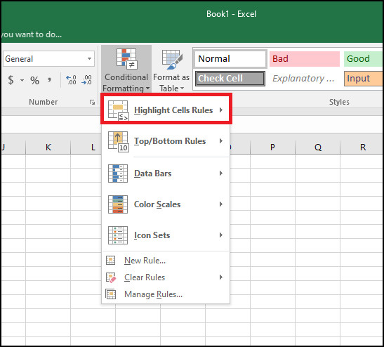
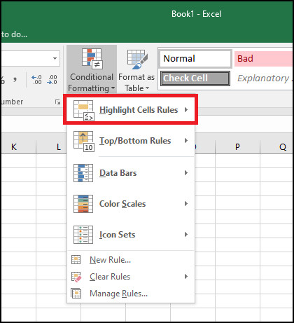
- Select Highlight Cell Rules from the menu.
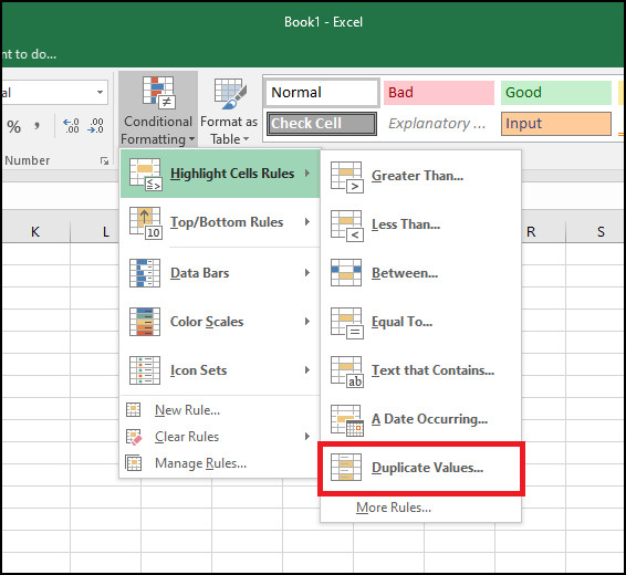
- Click on Duplicate Values.
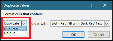
- Select Duplicate from the left list.
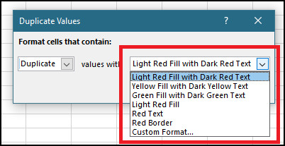
- Choose your desired highlighting format from the list on the right.
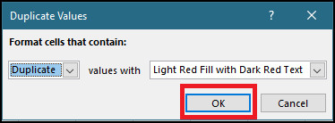
- Click on OK.
After you have gone through the steps mentioned above, the duplicate data will be highlighted according to your selected formatting style on that column, making it easy for you to find duplicate cells.
You can then select duplicate values and manage them however you want to. The common thing to do is to remove duplicate values after selecting the highlighted cells containing them.
2. Highlight duplicates in multiple columns
Instead of one single column, if you want to highlight the identical data existing on a number of columns, you can also do it by highlighting duplicate values with conditional formatting as before.
To identify and highlight the duplicates in multiple columns, follow this process:
- Open the spreadsheet you are working on using Microsoft Excel.
- Use Ctrl + Left Click to select the top of the columns that you want to highlight duplicates from.
- Open the Conditional Formatting menu.
- Select Highlight Cell Rules from the expanded menu.
- Click on Duplicate Values.
- Select Duplicate from the left list.
- Choose your desired highlighting format from the list on the right.
- Click on OK.
Following these steps will then highlight similar data according to your chosen format on the columns that you have selected during the process. You will see them highlighted with the color and format you have chosen, be it a red fill or dark red text.
1. Find out and highlight duplicate rows in Excel
There are some cases when the same row of data has been entered into a spreadsheet and needs to be found out to remove because of appearing multiple times. If you want to check for duplicate rows, you cannot use the method mentioned earlier. You have to take the help of the textjoin and countifs functions.
When you want to find out and highlight the same rows, firstly, you will have to group all the data in the rows on a separate column using textjoin and then highlight the same data by using that column and making a custom formatting rule to identify duplicates using countif function.
Go through this process to find the duplicate data rows and highlight them:
- Open your spreadsheet in Microsoft Excel.
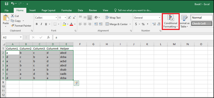
- Create a new helper column to find same rows.
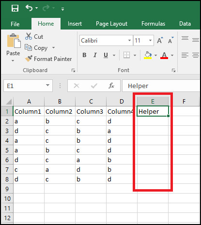
- Type in =TEXTJOIN(“,”,TRUE,A2:D2) on the first cell of the new column.(The red part is the range of cell which will be different in your case. Check image to compare)
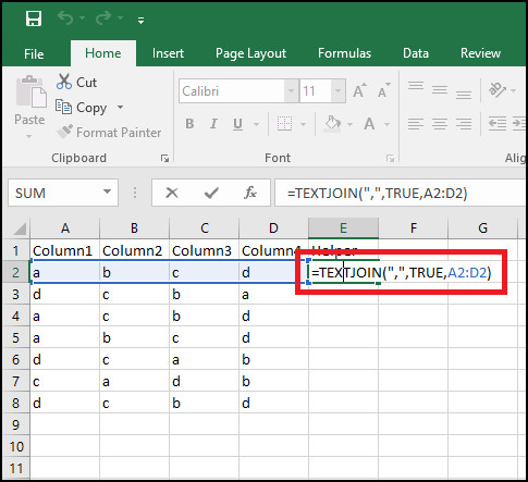
- Put that value in all the cells of the new column.
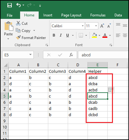
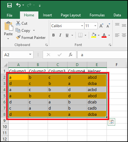
- Select the data range containing your values other than the headers.
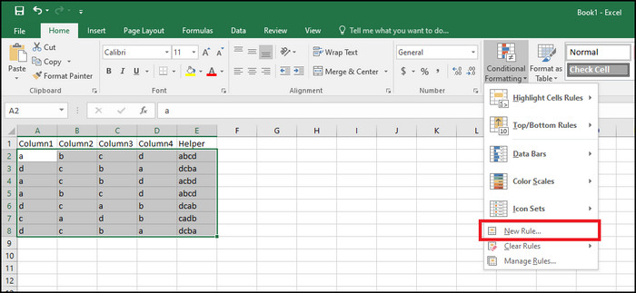
- Open Conditional Formatting menu in the home tab.
- Select New Rule option from the expanded menu.
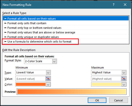
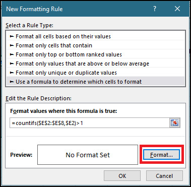
- Click on Use a formula to determine which cells to format.
- Type in this formula: =COUNTIFS($E$2:$E$8,$E2)>1 on the given space under Format values where this formula is true.(The red parts will change in your case. Refer to given image to compare)
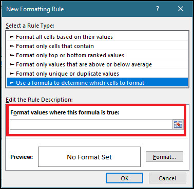
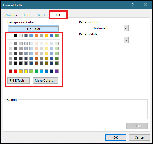
- Go to Format.
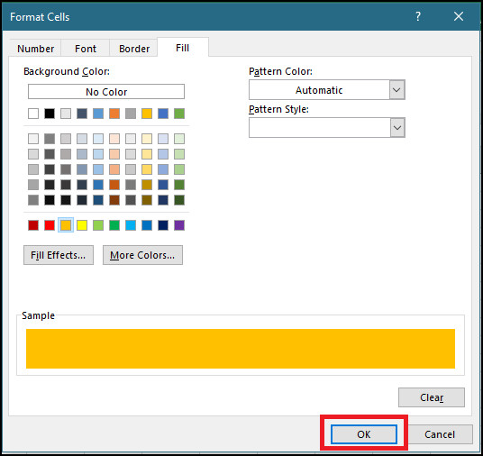
- Choose your highlighting color under Fill tab.
- Click on OK.
- Select OK again on New Formatting Rule window.
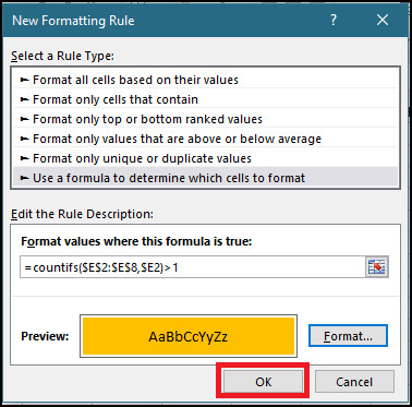
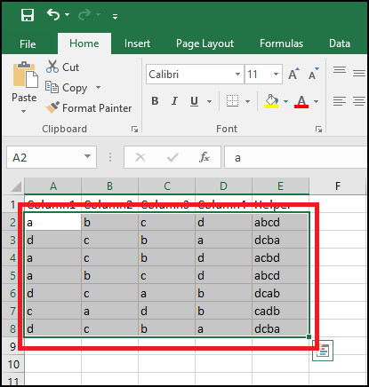
After you have done this, you will see that the same rows of your selected range of cells on your worksheet have been highlighted by your selected color. 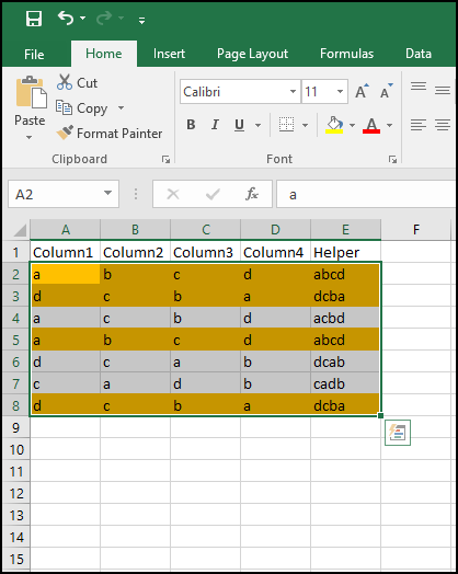
How to remove duplicate rows in Excel?
By now you know how to highlight the duplicate entries in your sheet but how are you going to manage them?
If you want to remove these entire duplicate rows of data from your spreadsheet, you can also easily do it in Excel after you find duplicate values using the helper column.
This is how you can remove duplicate rows from Excel:
- Find out your duplicate rows by using the helper column method.
- Select all the cells that have your data.
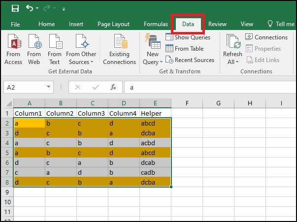
- Go to the Data tab.
- Click on Remove Duplicates.
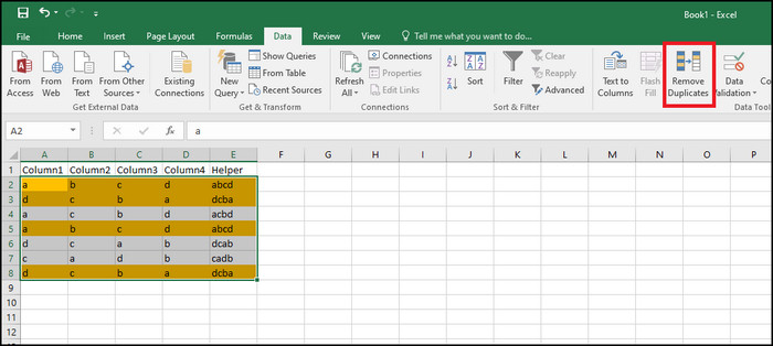
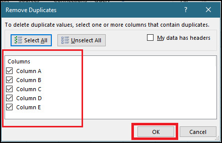
- Select the columns to remove duplicates from and click on OK.
After taking these steps, you will then see that all the duplicate rows that appeared multiple times within your dataset have been removed, leaving only one copy of those rowss. 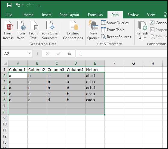
Conclusion
Working on spreadsheets means working with large amounts of data at once and MS Excel provides its users with some amazing and resourceful tools to manage that data.
The same data can exist multiple times within a spreadsheet because of being mistakenly entered many times or any other hitch. Being able to highlight those extra entries lets Excel’s users easily detect and deal with them efficiently in a short amount of time.
Checking out the methods of highlighting duplicates in the Excel spreadsheets that are presented in this guide will allow you to apply those methods like a pro.
Dealing with duplicates will then be only a matter of a few clicks for you.