A worksheet with lots of data is hard to read and focus on.
That’s why Microsoft Excel has the option to create outlines, group rows, and columns along with a single click expand-collapse.
It’s an essential feature that’ll make large worksheets with multiple levels of data easier to read.
This post will guide you through the process of grouping rows in Excel, both manually and using the outline option.
You’ll learn about nested groups, group by features, and grouping PivotTable.
You’ll also know how to undo these options (ungroup, remove outline) and expand-collapse.
So keep reading the post till the end.
How To Group Rows In Excel
There are two main methods to group rows in Excel: automatically (using the Outline option) and manually (using the Group option).
You can also use the Subtotal option and group rows in PivotTable.
Follow the methods below to group rows in Excel:
1. Use the Outline feature (Automatic Grouping)
Microsoft Excel has the Outline option, which allows you to create single-level groups automatically.
The Outline cannot group data based on multiple columns (i.e., it cannot create multi-level groups). It only works with single-level data, and Excel should be able to detect it.
In this example, I have a worksheet containing AMD CPUs from both desktop and mobile platforms.
Notice I have two summary rows: “desktop total” and “laptop total,” which correspond to the total sales figure of each platform CPUs.
Also read how to freeze panes in Excel easily.
Your worksheet must have a similar summary row for each data category (in my example, I have summary rows for desktop sales and laptop sales categories).
The Outline option in Excel depends on the summary row to group rows. Without the summary row, you’ll see an error message “cannot create outline.”
Once you have the summary row ready (sum of sales, sum of profit, or anything similar), you can proceed to group rows.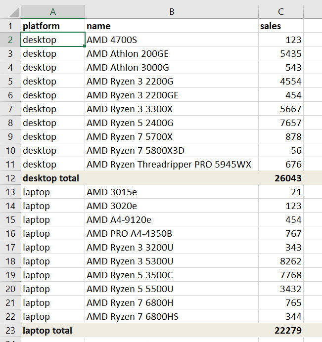
Here are the steps:
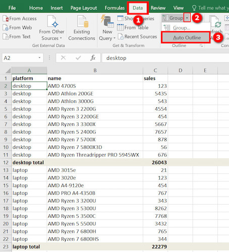
- Select any cell of any row you want to group.
- Switch to the Data tab from the top.
- Click on the arrow beside the Group option in the top ribbon.
- Select Auto Outline.
You’ll now see the worksheet grouped by rows according to the summary rows. The number of groups will correspond to the number of summary rows (one group for each summary row). 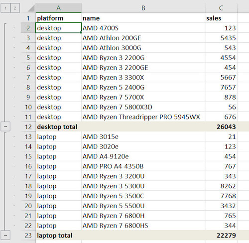
By default, Excel expects the summary rows below each row group (as in my example). In case your summary rows are located above each group, click on the arrow bottom-right of the Outline group in the ribbon, then untick the “summary rows below detail” checkbox, and click OK. 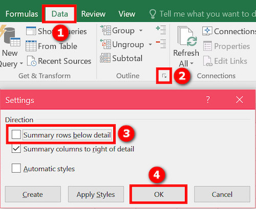
On the left, you can see the bars which highlight each group.
The minus button for each group will collapse the group rows and only show the summary row.
When you collapse a group, a plus button will appear for the group. Clicking on the plus button will expand the group.
You can also collapse or expand a group by selecting a cell in the group, then using the hide details or show details button respectively on the top ribbon.
On the top-left of the worksheet, you’ll see two gray buttons labeled 1 and 2. Clicking on 1 will expand-collapse all the group rows (and only show the summary rows). Clicking on 2 will expand-collapse all the rows. 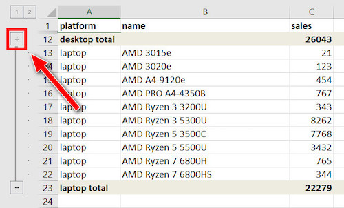
That’s how you can group rows in excel with expand-collapse on top.
2. Create nested groups (Manual Grouping)
You’d need to create nested groups if you have nested summary rows.
Excel doesn’t have an option for the automatic creation of nested groups. Hence you need to do it manually.
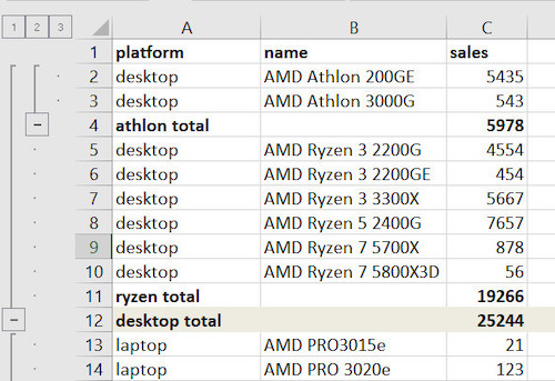
In my example, I have now created four more summary rows: two inside the desktop platform (Athlon total and Ryzen total) and two inside the laptop platform (PRO total and Ryzen mobile total).
Once you have a similar worksheet containing nested summary rows, do as follows:
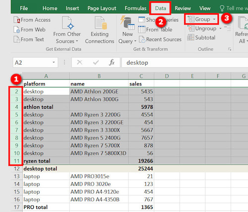
- Select all the rows in an outermost group (in my case, I selected all the desktop rows, excluding the desktop total summary row).
- Switch to the Data tab at the top.
- Click on the Group button. Alternatively, use the shortcut Shift + Alt + Right arrow.
- Select Rows if you’re asked about the group direction.
- Notice the bar on the left, which highlights the group.
 Since I have two outer groups (desktop and laptop), I’ve created another outer group for the laptop platform in the same manner. Now it’s time to create the inner groups.
 - Select all the rows of an inner group (I’ve selected all the desktop Athlon CPU rows up to the “Athlon total” summary row).
- Click on the Group button (or use the Shift + Alt + Right arrow shortcut).
- Repeat the steps for each inner group.
- Work your way from the outermost layer to the innermost one to create nested groups.
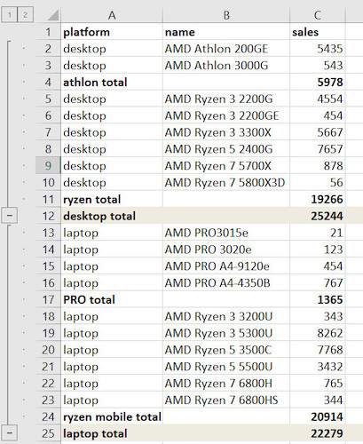
In this way, you can create nested groups for multi-level data. I’ve created 3 level groups. The first level corresponds to desktop and laptop total. The second level corresponds to all the inner summary rows (Athlon total, Ryzen total, PRO total, and Ryzen mobile total). The third level corresponds to all the rows. 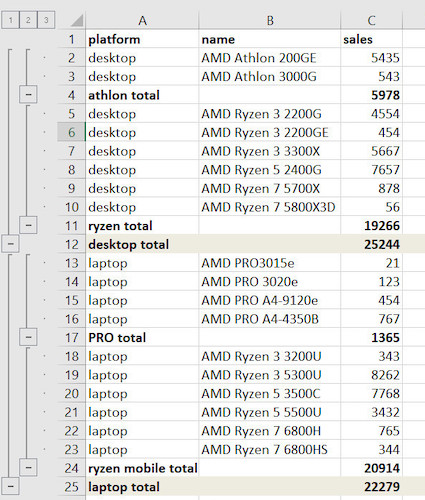
To expand and collapse groups of a particular layer, click on the “+” (expand) or “-” (collapse) button corresponding to the group on the left. 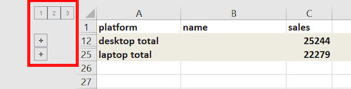
To expand and collapse an entire level, use the numbered buttons (1, 2, 3) on the top-left corner. 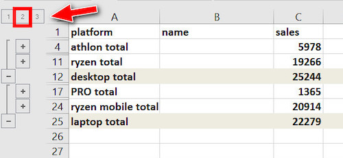
It allows you to collapse a large data set and only focus on the one you’re currently interested in. The data becomes more readable and easy to analyze the summaries.
That’s how you group rows on Excel and expand and collapse.
3. Group PivotTable
You can group rows in Excel PivotTable to make them stand out in large data.
The PivotTable grouping option has some neat options to group rows in excel based on cell value.
If the value is a date, you can group rows by days, months, quarters, etc. If the value is a number, you can set an interval for each group.
Here are the steps to group rows in PivotTable:
- Right-click on a cell containing a value you want to group by.
- Select Group.
- Select the “Starting at” and “Ending at” options, and edit the value.
- Choose how you want to group the values (month, quarter, years, etc. for date and interval value for numbers) in the “By” section.
- Click on OK to confirm.
To rename the group, go to Analyze > Field Settings from the top ribbon.
Here is the easiest guide to lock a cell in Excel.
4. Use the Subtotal option (automatic grouping)
An alternative to the Outline option is Subtotal. Subtotal has the same effect as Outline.
In fact, Subtotal is more advanced than Outline as it will create the summary row alongside grouping rows. Excel functions like SUM, COUNT, AVERAGE, etc., are available to generate the summary row.
When using Outline, you needed to create the summary rows yourself. When using Subtotal, you need to sort the column the groups will be based on.
Also, you can create nested groups using the Subtotal option. The only catch is that the column needs to be sorted correctly.
Here are the steps:
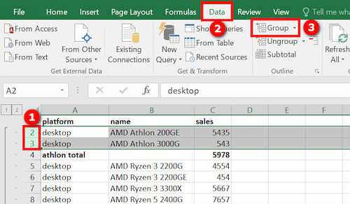
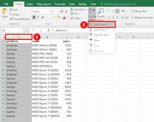
- Sort the values of the column upon which you’ll group. In my case, I’ll sort the “platform” column as I’ll make groups of platform-wise sales (notice carefully that I’m not sorting the “sales” column).
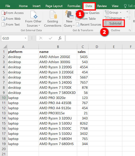
- Switch to the “Data” tab.
- Select a cell in the column upon which you’ll group. I’ll select a cell in the “platform” column.
- Click on the “Subtotal” button in the Outline ribbon. The Subtotal dialog box will appear.
- Select the column that you want to group by in the “At each change in” drop-down. In my case, I’ve selected the “platform” column.
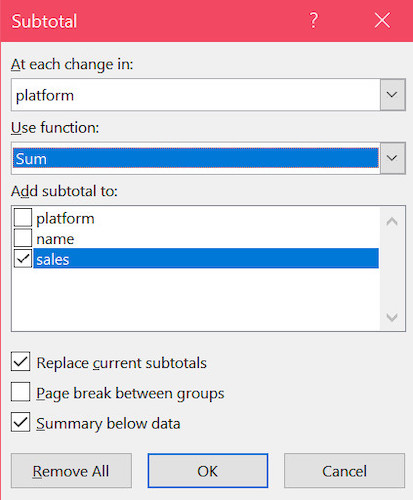
- Select the Excel function in the “Use function” drop-down, which will be used to generate the value in the summary row. I’ve selected the SUM function since I’m interested in the total sum of sales.
- Select the column in the “Add subtotal to” drop-down from which the values will be used to calculate the value of the summary row. I’ve selected the “sales” column as the sum of sales value is used to generate a summary row for each platform (notice how it differs from the first drop-down).
- Choose if you want the summary below or above the data.
- Select OK to group the rows.
Now you’ll see the bar on the left for each group as well as an outer bar for the grand total summary row. 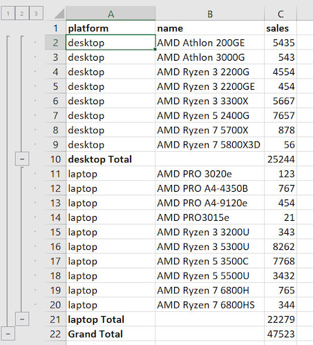
Here I have grouped the rows of each platform (hence sorted the platform column and also selected it in the “At each change in” drop-down) for total sales (hence selected the sales column in the “Add subtotal to” drop-down).
If I were to count the number of CPUs in each platform, I’d sort the data by “platform” and select the platform column in both the “At each change in” and “Add subtotal to” drop-down. Instead of the SUM function, I’d use the COUNT function. 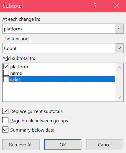
The result would look like this. 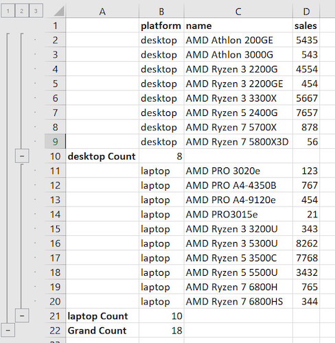
Follow our ultimate guide if you want to know how to post Bank Statement in Excel to Quickbooks.
How To Remove Groups In Excel
Removing groups in Excel is more straightforward than creating them.
Here are the different ways to remove groups based on how they’re created:
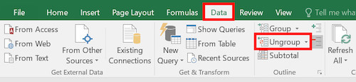
- Outline: Switch to the Data tab, then click on the arrow beside Ungroup button. Select “Clear Outline“.
- Nested groups (manual): Select the rows you want to ungroup, then go to the Data tab and click on the Ungroup button.
- PivotTable: Right-click on any cell in the group, then select Ungroup.
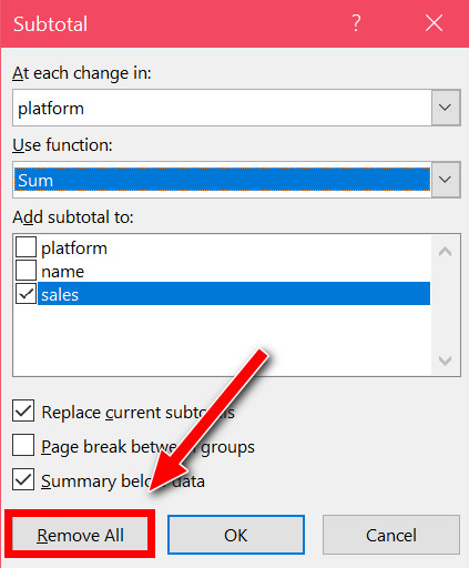
- Subtotal: Select a cell in the column where the Subtotal was performed. Then go to the Data tab and click on the Subtotal button from the top ribbon. The Subtotal window will appear. Click on the Remove All button to remove the Subtotal grouping.
Your data will not be deleted when you remove groups.
Also read how to shade every other row in Excel.
Final Thoughts
Grouping rows of cells in Excel helps you perform more tasks in a small time as it’s easy to analyze and work with data in segments.
Creating groups helps you to collapse groups that you don’t currently need and only focus on those you’re working with.
You can create groups using the Outline or Subtotal option or create groups manually using the Group button. PivotTable also has grouping functionality.