Although Microsoft Excel offers a great way to get a predictive value from any data set, you have to know exactly which function to use to get the best-fit curve.
For example, you can’t just apply linear functions to use non-linear interpolation in Excel. To do that, you have to follow a few precise steps to get your desired chart, which I have thoroughly addressed in this write-up.
So, without wasting any more time, let’s discuss the best approach for non-linear interpolation in Microsoft Excel.
What is Non-Linear Interpolation and Can We Do It in Excel?
Non-linear interpolation is a process of estimating unknown values between two known data points when the relationship between the data points is not linear. In short, it’s a prediction method that uses available non-linear data points to determine the next values.
For example, if you have a table of values for the height and weight of some people, you can use non-linear interpolation to estimate the weight of a person with a given height that is not in the table.
And to address the second query: Yes, we can do non-linear interpolation in Excel, but the approach is quite different than linear interpolation.
Fortunately, Microsoft has provided different ways to perform such tasks depending on the type and amount of available data.
How to Use Non-Linear Interpolation in Excel
Linear and non-linear interpolation requires completely different Excel formulas. For linear interpolation, the LINEST or FORECAST functions can do the trick. But you can’t use them for non-linear data sets as they won’t yield the best-fit curve.
If the values in your Excel data table do not have a constant rate of change or a constant slope, you need to use polynomial interpolation functions, like GROWTH or TREND, to derive interpolated values.
Below, I have explained the whole process in great detail. So read on and don’t skip over any crucial steps.
Here’s how to use non-linear interpolation in Excel:
1. Use the GROWTH Function
In Microsoft Excel, the most commonly used function for non-linear interpolation is =GROWTH(known Ys,know Xs,new Xs,constant). Here, the constant is usually set as 1 to derive the adjacent values.
So, to use the GROWTH function:
- Plot the data table into your Excel spreadsheet. Refer to the attached example image if needed.
- Select the cell where you want the interpolated value to be. For demonstration, I’m selecting the H17 cell.
- Type =GROWTH( and select the known Y values/dependent variables. For me, they’re located in I4 to I15 cells. After selecting the range, it should look like I4:I15 in the formula.
- Input a comma(,) and select the known X values/independent variables from H4:H15.
- Type a comma again and select the cell with the lookup value. For me, it’s H17.
- Input a comma and type 1.
- Close the bracket and press the Enter button on your keyboard. The final formula should look something like this: =GROWTH(I4:I15,H4:H15,H17,1).
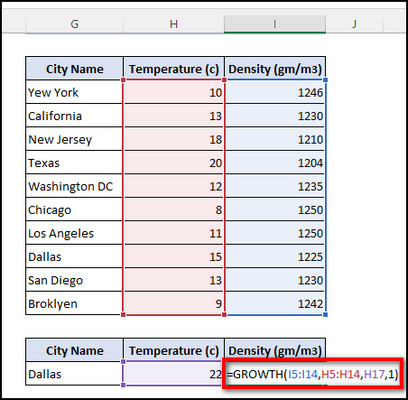
Voila! You’ll see the interpolated value in the H17 cell.
2. Use the TREND Function
The TREND function uses a similar kind of formula as the GROWTH function, which is =TREND(known Ys,known Xs,new Xs,constant). So, for our reference table, the non-linear interpolation formula stands as: =TREND(I4:I15,H4:H15,H17,1).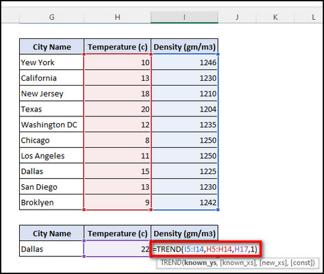
Now, hit the Enter button, and you’ll get the same result as the previous method from this non-linear interpolation formula.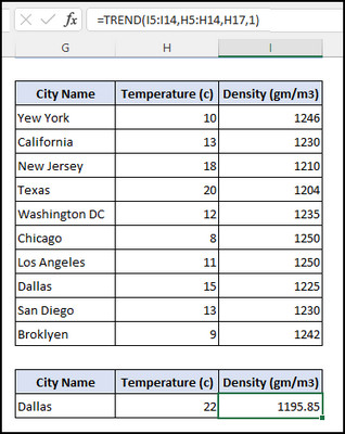
Now, if you’re interested in 3D interpolation in Excel, don’t forget to check out the embedded article.
How to Use Trendline to Get a Non-Linear Interpolation in Excel
In addition to performing non-linear interpolation, Excel also has the trendline feature to visually represent the interpolation trend as a curve.
Follow these steps to use trendlines for non-linear interpolation in Microsoft Excel 365:
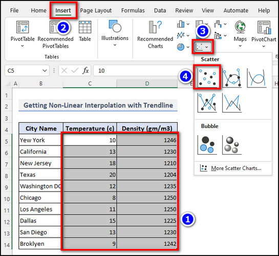
- Select all the cells for both X and Y values, like C5:D14.
- Go to the Insert tab.
- Select Scatter chart type from the Charts sections.
- Click on the plus icon next to the chart and tick the box for Trendline.
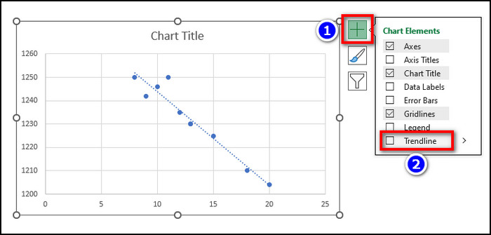
That’s it. The chart should look something like this: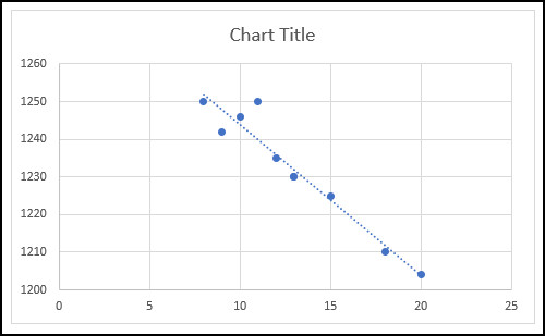
This way, adding a trendline in Excel chart can help users identify any inconsistencies or exceptions in the values and modify the interpolation as needed.
Also, there are Excel interpolation add-ins like Solver tool or other third-party plug-ins that can serve the same purpose.
Bear in mind, non-linear interpolation and non-linear regression are not the same, as they have different goals and assumptions.
Wrapping Things Up
Correctly plotting the data values and using the GROWTH or TREND functions is the best approach to interpolate data in Excel using non-linear regression. And following this article is the best way to learn how to do so.
Anyway, that’s it for today. For any further assistance on any MS Excel or any other Microsoft services, don’t forget to check out the extended guides on our website.
Have a good one!