In a corporate environment, it’s pretty common to have a ton of data in an Excel sheet is pretty common. Nonetheless, this makes it extremely difficult for an employee to find a specific value from that bloated spreadsheet.
Although Microsoft has provided built-in functions to check if a value is in a list in Excel, the key is to know how to apply those formulas properly, which I have thoroughly discussed in this article.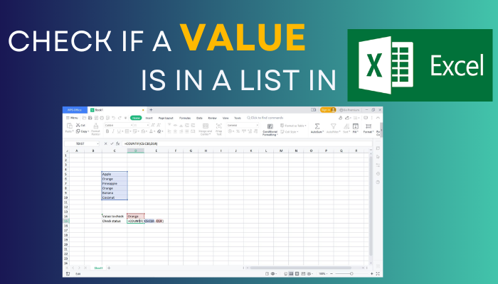
So, without any delay, let’s get started.
How to Check if a Value is in an Excel List
In order to check if a text is in a list in Excel, selecting the data range and using the COUNTIF function is the most commonly used technique. But that’s not all! There are some other useful functions that can serve the same purpose but in a different manner.
Not to mention, the built-in Find & Select feature offers an effortless way to quickly check if a product name is in the Excel list. However, every option/function has some limitations.
What can you do when you want to search for a value but only remember a portion of it? Or what about when you want to search multiple keywords?
To address every scenario, I have shortlisted the most precise methods to find your desired outcome and explained how to use the functions accordingly. You can pick any of the below-listed processes or choose a specific one that serves your purpose.
Here’s how to check if a value is in a list in Microsoft Excel:
1. Use the Built-in Find Option
For the most part, we can use Excel’s Find feature to check if & where a certain keyword exists in a data entry. Here’s how:
- Open your Excel data sheet and click on the Home tab.
- Choose Find & Select from the Editing section.
- Click on Find > Options.
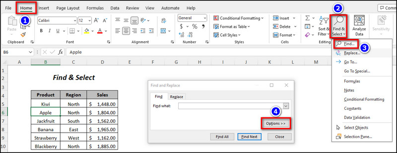
- Keep Within, Search, and Look in options to their default values, which are Sheet, By rows, and Formulas. If these aren’t the default settings, change them accordingly.
- Type the text you’re looking for in the Find what box and click on Find All.
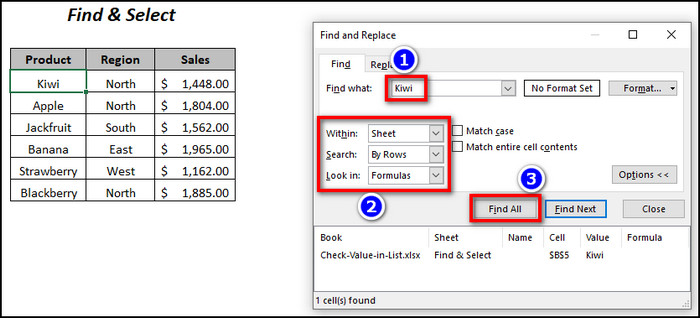
That’s it. You’ll be redirected to the cell on your Excel sheet where that value is located. For example, I searched for Kiwi, and it showed the result and its cell position, which is B5 in the sheet.
2. Apply the COUNTIF Function
The COUNTIF function does exactly what the name suggests: it counts all the cells to find out how many met the set condition. If it finds the suggested value, it’ll show TRUE. If not, it’ll return FALSE.
Here’s how this works:
- Select the cell range where you want to find the value. For demonstration, I’ve selected N5:N10.
- Input the value that you want to find in Q5 and select the R5 for the output cell. In this case, I want to find the product Kiwi, which I’ve placed in Q5.
- Type =COUNTIF($N$5:$N$10,Q5)>0 in the R5 cell and hit Enter. Change the value in the bracket according to your sheet.
- Check if the cell shows TRUE or FALSE.
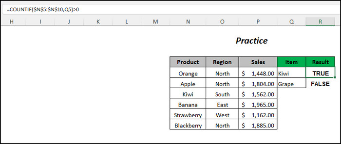
As we can see, since my data table has Kiwi in it, the message reads as TRUE. Let’s say we search for Grape, placed in the Q6 cell, and type =COUNTIF($N$5:$N$10,Q6)>0 in the output R6 cell; it’ll come back as FALSE.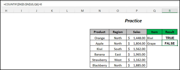
3. Combine IF and COUNTIF Functions
If the TRUE or FALSE sounds too vanilla for you, there’s a way to display a custom text, like Yup or Nope. To do so, you have to use the previously mentioned COUNTIF with the addition of the IF function. Here’s how:
- Click on the output cell and type =IF(COUNTIF(.
- Select the data range, like N5:N10, and give a comma.
- Choose Q5 or the cell containing the value you’re looking for.
- Close the bracket and type >0,”Yup”,”Nope”). So the full formula stands as =IF(COUNTIF(N5:N10, Q5)>0,”Yup”,”Nope”).
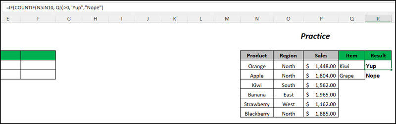
Done! Now press Enter, and you’ll either get Yup or Nope, depending on whether the value is in the list or not.
4. Use MATCH and ISUMBER Functions
The MATCH and ISNUMBER functions can also be used to perform the task at hand.
To check a value’s existence in an Excel sheet using this function, type the =ISNUMBER(MATCH(Q5,$N$5:$N$10,0)) formula in the output cell and hit Enter. Change the data range and the target cell accordingly.
As shown in the demo, for Kiwi, it shows TRUE as it exists in the list, and for Grape, it shows FALSE as it doesn’t.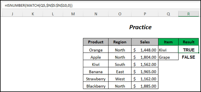
5. Apply Additional Operators to Check Partial Match
Suppose we want to find Berry from the list, but there are no standalone Berry product names in the Excel sheet. However, there are Strawberry or Blackberry, which partially matches the desired value.
So, what can we do to get the partial match? Because if we use the previous approaches, it will show FALSE or Nope.
To check for a partial match, type the desired value(Berry) in the Q5 cell and input the =IF(COUNTIF($N$5:$N$10,”*”&Q5&”*”)>0,”Matched”,”Not Matched”) formula in the output cell.
Here, $N$5:$N$10 denotes the cell range, and Q5 is the target cell where the search value is located.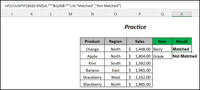
Now, press the Enter button on your keyboard. When the number of cells containing a partially matched value is greater than 0, you’ll get Matched. If not, you’ll see Not Matched.
6. Use OR Function
Just like the COUNTIF function, the OR function glances through the selected cells in your Excel data table and shows TRUE or FALSE, depending on the availability of the desired value.
To use this function, input the value you are looking for in the Q5 cell and type =OR($N$5:$N$10=Q5) in the output cell. Change the parameters according to your Excel list.
Now, hit Enter, and that’s it. Considering the number of cells containing the desired value is greater than ), you’ll see TRUE. Otherwise, you’ll get the FALSE message.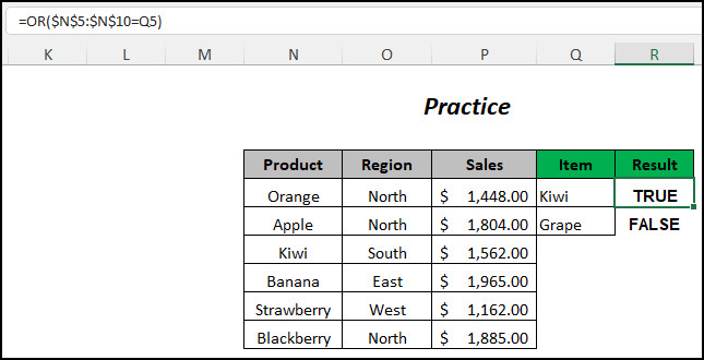
7. Use ISERROR, NOT, and XLOOKUP Functions
What if you want to find a specific product name from two individual ranges of cells?
In that case, you have to combine the NOT, ISERROR, and XLOOKUP functions and apply them properly. To do that, type =NOT(ISERROR(XLOOKUP(Q5,$N$5:$N$10,$O$5:$O$10))) in the output cell and hit Enter.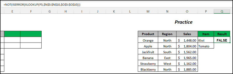
In the formula, the Q5 is the cell containing the desired value, $N$5:$N$10 is the first cell range/lookup array, $O$5:$O$10 is the return array. If the value is found, you’ll get the TRUE result. Otherwise, you’ll get FALSE.
8. Use a Combination of Functions to Find Multiple Values
When you want to find multiple values altogether from your Excel sheet, you’ll need to bring out the big gun. In this case, it’s the big formula.
Considering you’ve typed the desired values, separated by commas, in the M13 cell, type =IFERROR(INDEX($M$5:$M$10, SMALL(IF(COUNTIF(M13, “*”&$M$5:$M$10&”*”), MATCH(ROW($M$5:$M$10), ROW(M5:M10)), “”), COLUMNS($M$13:M13))), “”) in the output cell.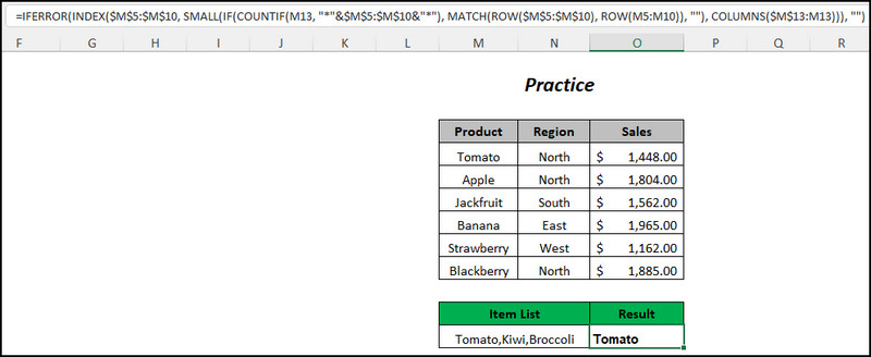
Now, press Enter, and you’ll see the value(s) that was found in the Excel list.
Final Thoughts
To be blunt, checking if a value is in a list in Excel using functions may sound more complicated than the built-in Find feature, but formulas give you much more flexibility to fine-tune your search.
That being said, I hope this write-up has provided you with the best-suited method for your work case. If you ever need further help on any Microsoft services, don’t forget to check out our website.
Have a great day!