750 million! Yes, you heard it right, that many users use MS Excel regularly. Excel is well ahead in the Spreadsheet business for its easy-to-use features.
You can quickly build your required charts and tables with the help of this Excel app. 
However, sometimes we deal with a lot of information while using this program. In those cases, shading every other row can help make our sheet more attractive and readable.
But many of you wonder how to shade rows in Microsoft Excel. It’s pretty easy. After investigating profoundly, I sort out some simple yet working methods like MOD or ODD/EVEN formulas that will help you color every other row in Excel.
Without skipping any part of this article, read along if you want to know. Let’s start!
How to Shade Every Other Row in Excel on Windows & Mac
If you want to shade or color every other row in Microsoft Excel, there are several methods. But the Table Format and the MOD formula are the most popular.
Additionally, I added the ISODD/ISEVEN formula in this content to assist you. Let’s head out and see how you can use those stated ways to complete the shading process.
Here are the steps to shade or color every other row in Microsoft Excel:
1. Apply the Table Format 
To apply the shade in rows, you can easily create a table from the specific chart. Building a table from the chart is the simplest yet functioning way.
Here are the steps to apply the table format on MS Excel:
- Open the MS Excel program.
- Compose your specific Excel sheet.
- Select the entire chart that you want to change.
- Move to the Home menu.
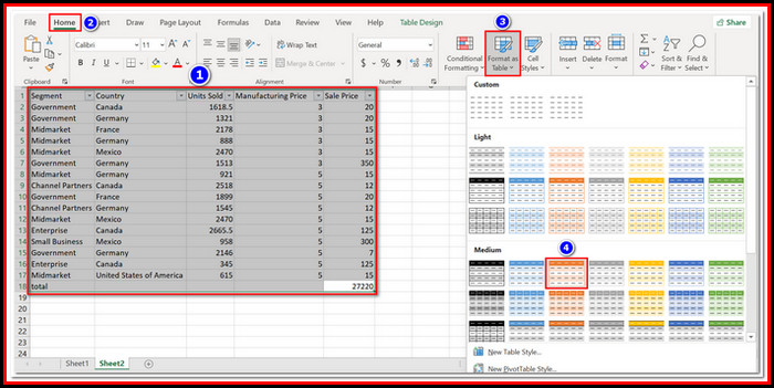
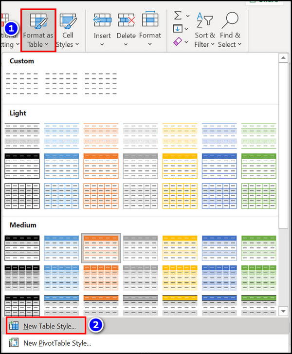
- Click on the Format as Table option.
- Choose your desired Format. You can select the New Table Style box if you want to modify the table.
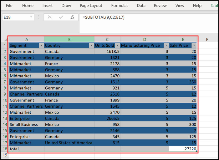
After choosing your specific Table format, you will see that the selected chart is converted into a nice row-shaded table.
Check out our latest fix for, how to Freeze Panes In Excel Easily.
2. Use the MOD Formula in the Conditional Formatting Option 
Using the MOD formula in the Conditional Formatting option is another way to complete the shading process in Excel. Users who want to use a formula in their Excel sheet can apply it to complete the shading process more conveniently.
Here are the steps to use the MOD formula in the Conditional Formatting option:
- Launch the Microsoft Excel application.
- Select the whole chart.
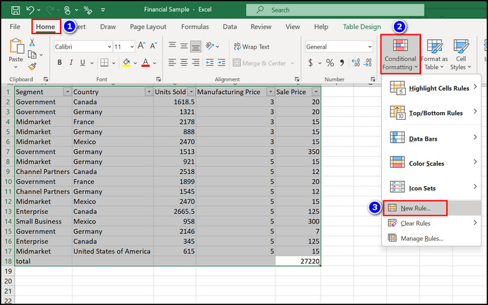
- Navigate to the Home section.
- Click on the Conditional Formatting option.
- Choose the New Rule option.
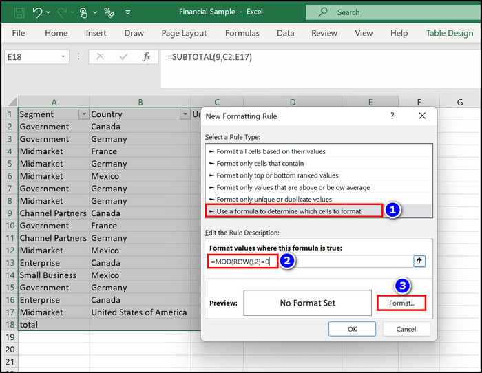
- Select the Use a formula to determine which cells to format option from the Select a Rule Type: box.
- Type =MOD(ROW(),2)=0 in the Format Values when this formula is true: box to add shade in every other row on MS Excel sheet. Additionally, if you desire to apply shade in every 3rd or 4th row, follow accordingly.
Type =MOD(ROW(),3)=1 formula if you want to apply shade every 3rd row. 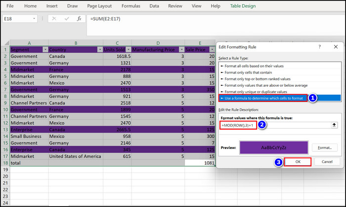
Write =MOD(ROW(),4)=1 formula to apply shade in every 4th row. 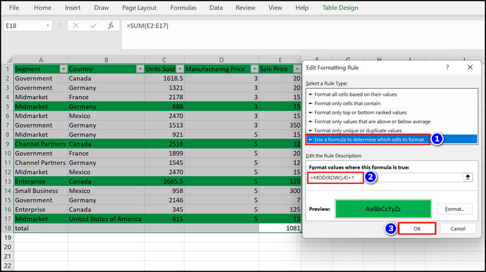
- Click on the Format button and select your specific shade Color, Number, Font or Border.
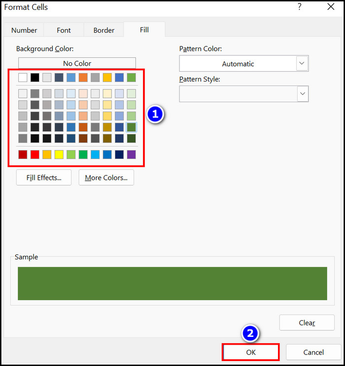
- Hit the OK button when color choosing is complete.
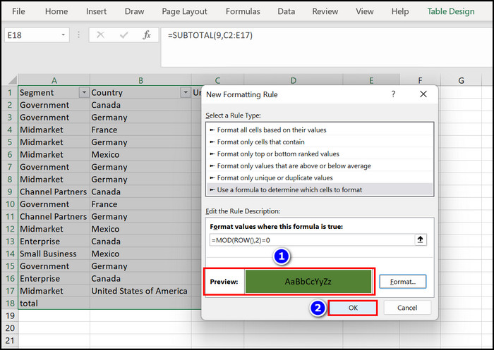
- See the Preview and hit the OK button.
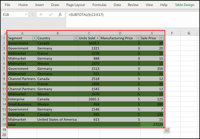
Immediately you will see that every other row is shaded with your desired color.
3. Use the ISODD/ISEVEN Formula on Conditional Formatting Option
Instead of using the MOD formula, you can apply the ISODD or ISEVEN formula to finish the shading process.
Let’s find out how to use the stated formula to highlight and color the even or odd number of rows in the Excel sheet.
Here are the steps to use the ISODD or ISEVEN formula to shade rows:
- Open the Excel app.
- Highlight the specific chart.
- Move to the Home section.
- Click on the Conditional Formatting option and select the New Rule option.
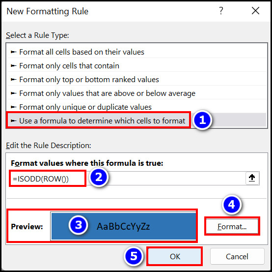
- Click on the Use a formula to determine which cells to format option.
- Write =ISODD(ROW()) formula in the Format Values when this formula is true: box if you want to apply shade to the odd number of rows.
- Type =ISEVEN(ROW()) formula in the box if you want to add color to the even number of rows.
- Click on the Format option and choose a specific color after typing the formula, then hit the OK key.
- See the Preview box and press the OK button.
The odd and even number of rows are shaded in your Excel sheet. Follow the next heading if you want to know how you can remove alternate row shading in Excel.
Follow our guide to fix, how to Lock a Cell in Excel.
How to Remove Alternate Row Shading in MS Excel
Removing the row shading or color from an MS Excel sheet is straightforward. Let’s see how you can finish this action without any hassle.
Here are the steps to remove row shading in MS Excel:
- Highlight the entire formatted chart from the Excel sheet.
- Navigate to the Home section.
- Click on the Conditional Formatting menu.
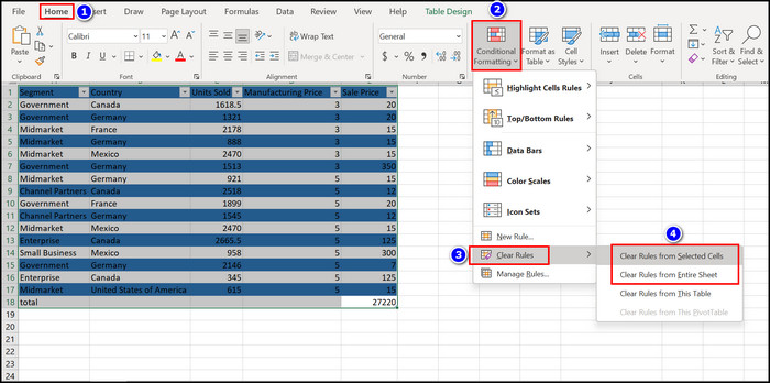
- Select the Clear Rules > Clear Rules from Selected Cells or Clear Rules > Clear Rules from Entire Sheet options.
Instantly, all the row shading or colors are gone from the sheet. Also, you can select the whole chart and follow the Home > Clear Formats options to remove the specific row shading from the Excel sheet.
Read the following heading if you want to shade every other column from the Microsoft Excel sheet.
How to Shade Every Other Column in MS Excel
In the previous segment of this article, I showed you how quickly you could add shade in Excel rows. But if you want to learn how to apply shade in every other column, follow the instructions below.
Here are the steps to shade every other column in MS Excel:
- Select the whole chart from the MS Excel spreadsheet.
- Click on the Home section.
- Choose the Conditional Formatting menu.
- Select the New Rule option.
- Choose the Use a formula to determine which cells to format option.
- Type =MOD(COLUMN(),2)=0 in the Format Values when this formula is true: formula box.
![shade-column-excel]](https://10pcg.com/wp-content/uploads/shade-column-excel.jpg)
- Click on the Format option.
- Choose your desired Color, Font, Border and Number and click on the OK button.
- Look at the Preview section; if all are set, press the OK key.
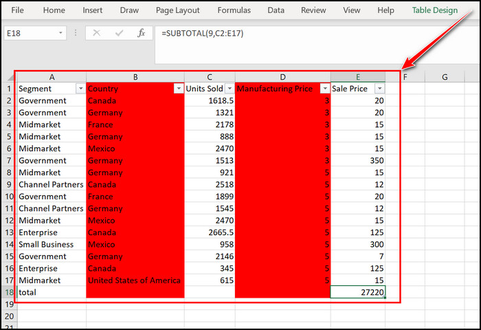
After pressing the OK button, you will notice that every other column is shaded with the selected color.
Also, don’t forget to check out our, Fix Microsoft Excel Freezing or Slow.
FAQs
Can you add multiple alternating colors in MS Excel?
Yes, you can add multiple alternating colors in the Microsoft Excel program. Move to the Home menu and select the desired color from the Fill Color option.
How do I highlight every other row in conditional formatting on Excel?
To highlight every other row in MS excel you need to follow Home > Conditional Formatting > New Rule > Use a formula to determine which cells to format > =MOD(ROW(),2)=0 > Format > Choose Color > OK options.
What are banded rows in Microsoft Excel?
The shaded or colored rows in a spreadsheet are the banded rows in Microsoft Excel.
Read more on, How To Highlight Duplicates In Excel
Final Thoughts
MS Excel is an incredible application that can help us to complete our specific tasks.
Shading or coloring every other row in Microsoft Excel is a simple process. You must use the MOD or ISEVEN/ISODD formulas to complete this operation smoothly. But if you don’t want to apply the formula, use the Table Format method.
Overall if you read this content carefully, you already know what options you have to finish the shading process. Also, this article teaches how to remove shading from Excel.
As always, it’s time to say goodbye. Let me know your afterthoughts about this article in the comment section.