Whether you are making a data sheet for products sold, a proposal for a project’s expenses, or even a simple invoice, multiplying the values of different columns in Microsoft Excel needs to be done for several purposes like these.
Excel does this job very well because that is what it was designed to do in the first place, allowing users to deal with numbers however they want. The technique of multiplying columns in Excel is one of the simpler tasks and it can be done in a few ways, which are presented here in easy words. After going through this guide you will be able to carry out column multiplication in Excel like a pro.
So keep reading if you want to know how to easily multiply columns in Excel.
Go and check our other article on change row height in Excel.
What Is The Multiplication Formula In Excel?
Microsoft Excel has formulas that are like commands that you can enter into cells to manipulate the values of that and/or different other cells. The formula for multiplying values of cells is =PRODUCT(cell1:cell2). This function can be used to multiply values from cells in different rows and columns.
By using the PRODUCT formula, you can multiply any number of cells on the same and different columns at a time.
The parentheses in the formula can contain a range of cells (cell1:cell2) or individual cell references separated by commas (cell1,cell2,cell3). It can also contain range of cells and individual cells together which also need to be separated by commas (cell1:cell2, cell3, cell4).
The PRODUCT formula will multiply the value of every cell within the cell range and also the individual cells within the parentheses altogether.
In Excel, you can multiply columns using the PRODUCT formula or you can also do it in other ways. All of these methods of multiplying columns have the same result and so, you can use any method of column multiplication that you prefer.
These techniques are all explained in the following section of this guide. So, move on to the next section to learn the ways of multiplying values within different columns in Microsoft Excel.
Here’s a complete guide on how to sort by date in Excel.
How To Multiply Different Columns In Excel
Microsoft Excel is an app that was built and optimized to deal with numbers as you please on your spreadsheet. For this, multiplication of columns can be done in a few ways in excel: by using multiplication symbol (*), by using the PRODUCT formula or by using array formula.
These three techniques of multiplying columns in Excel can be employed to multiply values in two or more columns however you want, depending on the purpose of your multiplication.
The ways column multiplication in Excel are straightforward processes. All of them are discussed in this section elaborately so that it is easy for you to grasp them and apply as a skill. It is up to you which method you want to apply because they are all means to the same goal, that is, to multiply values in two or more columns.
Follow these steps to know how to multiply columns in Excel:
1. Multiply Using Multiplication Sign (*)
Multiplying columns in Microsoft Excel can be simply done by using the multiplication sign (*) in the formula along with the cell references. For this you will have to create a new column to hold the results of your multiplication and type the formula there.
Here’s how you can multiply columns in Excel using multiplication sign (*):
- Open your spreadsheet file using Microsoft Excel.
- Create a new column beside the columns you want to multiply to hold your results.
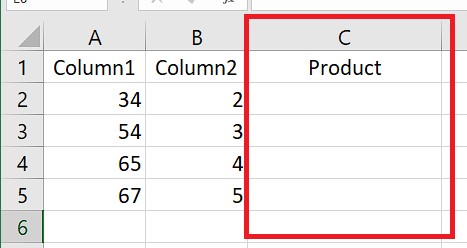
- Type in the following formula on the first cell of the new column:
=cell1*cell2 (for two columns) 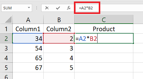
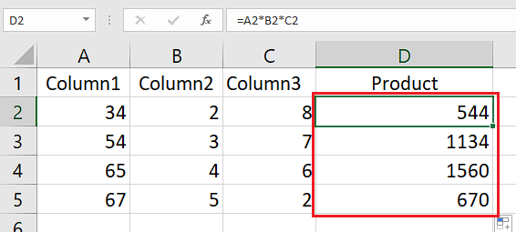
Or, =cell1*…*cell2 (for more than two columns) 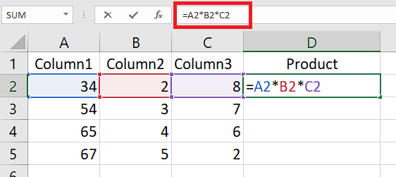
(cell1 and cell2 are first cells of the columns you want to multiply. You can multiply several columns in this way).
- Double-click on the cell filler icon on the bottom-right of your formula cell to fill all the cells on your product column.
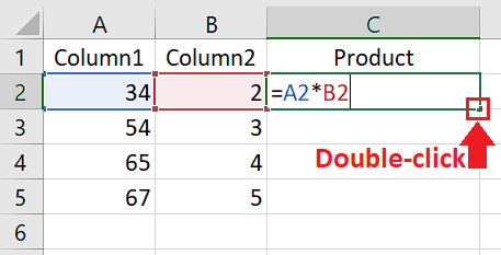
Since you have written the relative cell references in your formula on the first cell, they will be changed to the respective cell references corresponding to the later cells on your product column.
So, each cell of the new column will now carry the value of the product by multiplying each cells of your initial columns. 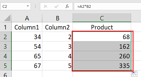
Check out the easiest way to do a subscript in Excel.
2. Multiply Using PRODUCT formula
The formulas in Excel are excellent tools for manipulating numbers. As you have seen earlier, you can also use the PRODUCT formula to multiply the values of two or more columns in Microsoft Excel.
This is how you can multiply columns using PRODUCT formula in Excel:
- Open your spreadsheet using Microsoft Excel.
- Create a new column beside the columns to be multiplied for holding your products.

- Type in the following formula on the first cell of the new column:
=PRODUCT(cell1:cell2) 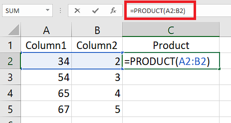
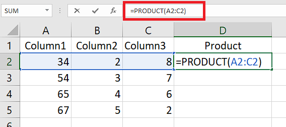
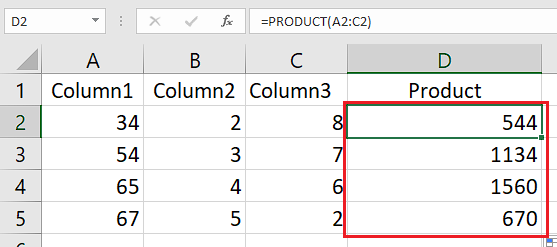
(cell1 and cell2 are first cells of the columns you want to multiply. Note that the columns you want to multiply need to be consecutive for this to work. You can multiply several columns where cell1 will be the first cell of first column and cell2 will be first cell of the last column among the consecutive columns).
- Double-click on the cell filler icon on the bottom right of your formula cell.
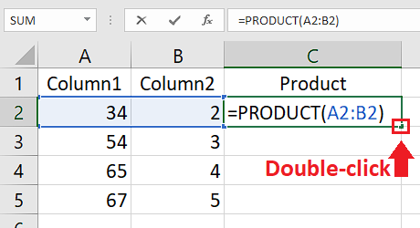
You will now have an entire new column with your desired products. Each cell in the new product column will contain the value of the product by multiplying their corresponding cells on your initial columns. 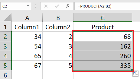
Follow our guide step-by-step to remove page break in Excel.
3. Multiply Using Array Formula
You can express the values of your column mentioning your column’s range within your formula (for example: A2:A5). You can employ this method with array formula and multiplication operator (*) to multiply columns in Microsoft Excel.
Go through this process to multiply columns using array formula:
- Open your spreadsheet on Microsoft Excel.
- Create a new column beside the columns to be multiplied for holding the products.

- Type in the following formula on the first cell of the new column:
=cell1:cell2*cell3:cell4 (for two columns) 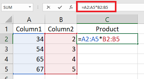
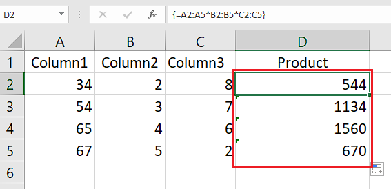
Or, =cell1:cell2*… : …*cell3:cell4 (for more than two columns) 
Here, cell1 = first cell of first column
cell2 = last cell of first column
cell3 = first cell of second column
cell4 = last cell of second column
- Press Ctrl + Shift + Enter to enclose the formula with { }. (DO NOT TYPE IN { } AROUND THE FORMULA MANUALLY)

- Double-click on the filler icon in the bottom-right of the cell.
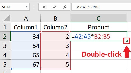
After you have taken these steps, you will see that you now already have your desired products on the new product column. 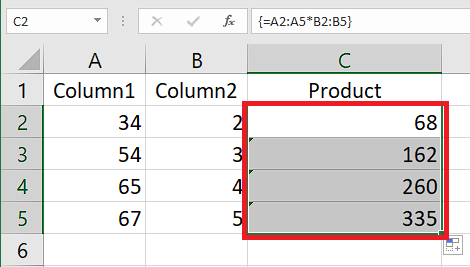
Check out our recent article on add months to date in Excel.
How To Multiply Columns With Constant In Excel
In the earlier methods, we have seen how to multiply the values in columns using relative cell reference. What if you have to multiply a constant number or an unchanged cell reference?
In these situations, there are two ways you could deal with them:
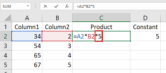
- You can enter the constant number directly on the formula multiplying with the rest of the part by the * sign.
- The constant value can exist within a separate cell on your sheet which you have to multiply using the absolute cell reference (e.g. $A$3) of the constant cell and the * sign.
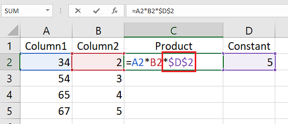
By using any of these procesudres of multiplying constants in an Excel formula, you can multiply your column’s values with any constant number.
Conclusion
Microsoft Excel is the ultimate tool to play with numbers on your worksheet and manage them in any way you please. You can freely multiply the values of any columns with with that of other columns in Excel very efficiently using the techniques that have been presented in this guide.
By familiarizing yourself with the methods of multiplying columns in Excel from here, you will be able to adopt this skill and apply it in an instant whenever you need to.
Multiplying columns in Microsoft Excel will then be a walk in the park for you.