There are several ways to count cells with multiple criteria in Microsoft Excel. Utilizing the PivotTables, COUNTIFS function, or conditional formatting is comparatively more difficult.
Fortunately, we can combine the advanced SUMPRODUCT and COUNTIF functions to count cells based on multiple criteria.
In this article, I will discuss the functions and show four methods of how to use these functions to count with multiple criteria.
So, let’s get started!
Understanding SUMPRODUCT Function
Let’s start the journey by understanding the SUMPRODUCT function. The default operation of SUMPRODUCT is multiplication. This function first multiplies the matching items of the selected ranges or arrays and then sums the values.
Consider the general syntax of the SUMPRODUCT function:
=SUMPRODUCT(array1, array2, …)
When you break down the formula, you will notice two primary parts. Here, =SUMPRODUCT is the main function, and array1, array2,… are the cell range in which the SUMPRODUCT function will multiply and then sum.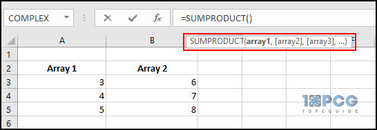
Allow me to show a real example to understand the function more precisely.
Suppose you’ve two arrays in your Excel file, and the cell ranges are A3:A5 and B3:B5, and you want to calculate the sum of the corresponding elements. In that case, you can use the SUMPRODUCT function to calculate the sum.
To do so, select an empty cell and type the following formula in the Excel formula box.
=SUMPRODUCT(A3:A5, B3:B5)
Once you press Enter, the formula will multiply the cell values (Column A x Column B) and then show the sum of the total values. In reality, this formula will perform the following calculation.
= (3 * 6) + (4 * 7) + (5 * 8)
= 18 + 28 + 40
= 86
And it will show the result 86. Now, move down to the next section to understand the COUNTIF function.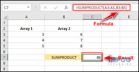
All About COUNTIF Function
COUNTIF is another unique function for calculating the number of cells from a cell range based on a particular criterion. This is essential to find the cells that contain specific information.
Following is the general syntax of the COUNTIF Function:
=COUNTIF(range, criteria)
Let’s break down the formula for a clear understanding. Here, =COUNTIF is the main function, the range is the number of cells, and finally, the criteria is the condition that determines which cells to count.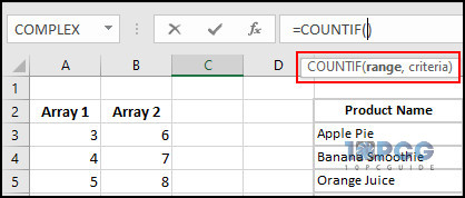
In Microsoft Excel, we can count regex with the COUNTIF function. Now, have a look at a real-life example of the COUNTIF function.
To count regular expressions (Regexs) with the COUNTIF function, select an empty cell and type the following formula in the formula box of Excel.
=COUNTIF(E2:E6, “*apple*”)
Whenever you press Enter, the formula will check the cells E2:E6 for the exact match of ‘apple,’ and the asterisk (*) will ignore all other text before and after ‘apple’ and finally show you the number of cells that contain the word apple.
As you can see in the above image, there are two cells with the word apple, and the COUNTIF function shows 2 in the result box.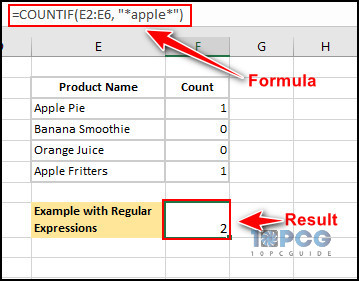
Now that we know all the ins and outs of SUMPRODUCT and COUNTIF functions, we can start using these functions to count cells with single or multiple criteria. For step-by-step instructions, jump to the next section.
How to Use SUMPRODUCT and COUNTIF Functions with Multiple Criteria
By combining the SUMPRODUCT and COUNTIF functions, we can count the number of cells in multiple ranges that meet multiple criteria. While the SUMPRODUCT multiplies true and false values, the COUNTIF function counts the actual number of cells that meet the criteria.
There are multiple fields when it’s necessary to combine the functions to count the cells accurately.
For instance, there aren’t many options in Excel to count cells with multiple criteria based on date. In such scenarios, the SUMPRODUCT and COUNTIF Functions come in handy.
Here are some examples of using SUMPRODUCT and COUNTIF functions:
1. Count Cells Between Numbers
If you want to get values from a specific cell range based on two particular values, you should combine SUMPRODUCT and COUNTIF functions.
For instance, we can get the number of students who scored more than 75 and less than 90. To do so, choose an empty cell and type the subsequent formula in the formula box.
=SUMPRODUCT(COUNTIF(D4:D13,”>75″))-SUMPRODUCT(COUNTIF(D4:D13,”>90″))
I know this formula looks quite complicated. Let me break down the formula so that you can catch the process efficiently.
Here, the COUNTIF(D4:D13,”>75″) part of the formula will calculate the cells D4:D13, which contain values greater than 75.
Similarly, the COUNTIF(D4:D13,”>90″) calculates the same cells but only accepts values less than 90.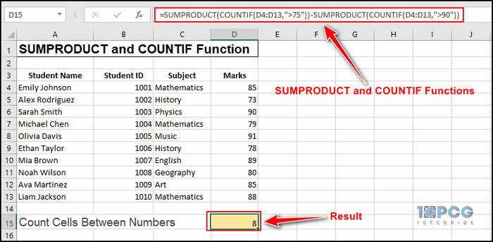
The entire formula calculates the values between 75 and 90 in the specified range (D4:D13) and shows the result 8 because it finds eight cells that meet the formula’s requirements.
That’s how you can use both SUMPRODUCT and COUNTIF functions to count the cells based on multiple criteria.
2. Find Text in the Same Column
Using the SUMPRODUCT and COUNTIF functions combo, you can also find text in the same column based on multiple criteria.
Let me clarify with an example: using this formula, we will count the occurrences of ‘History’ in the C4:C13 cell range. Simply click on an empty cell and use the following formula to find the text.
=SUMPRODUCT(COUNTIF(C4:C13,”History”))
In this formula, the COUNTIF(C4:C13, “History”) part is responsible for counting the number of cells that have an exact match with the word “History,” and the =SUMPRODUCT part is used to handle arrays more flexibly.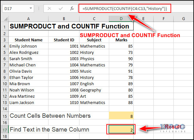
Once you apply this formula, it will check the cells C4:C13 and show you the selected cell’s total value (2). You can replace the criteria with any text that you want to count.
3. Count Cells Based on Dates
Using these functions, we can also count cells based on dates. For instance, we will count the exam date that was taken after 11/26/2023. We will apply the formula on multiple columns and calculate the cells that meet our criteria.
To begin the process, choose an empty cell as usual and then type the subsequent formula in the formula box.
=SUMPRODUCT(COUNTIF(C2:D31,”>11/26/2023″))
Here, the COUNTIF(C2:D31,”>11/26/2023″) part is doing the main calculations. Let me break it down to clarify the steps.
First, it will highlight the C2:D31 cells and then check if the cell values are greater than the criteria, which is 11/26/2023.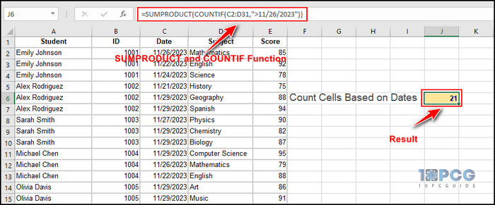
In this case, we have 21 cells after 11/26/2023; hence, the result is 21. The SUMPRODUCT function efficiently handles multiple columns so that the formula can generate accurate results.
4. Calculate Cells with Wildcard Operator
Alternatively, you can use these functions combined with wildcard operators to count cells with multiple criteria in multiple columns.
There are three different wildcards: Asterisk (*), Question Mark (?), and Tilde (~). In this method, I will show how to use the asterisk wildcard with SUMPRODUCT and COUNTIF functions to count cells that start with the character m.
To do so, click on an empty cell and type the subsequent formula in the Excel formula box.
=SUMPRODUCT(COUNTIF(A4:D13,”m*”))
Here, the COUNTIF(A4:D13,”m*”) part calculates the A4:D13 cells and finds the ones that start with m. As you can see, this formula checks multiple columns and uses the wildcard to count.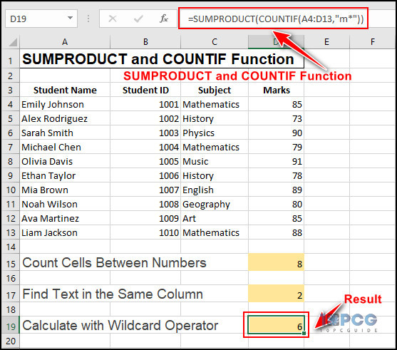
In the dataset, six cells start with m, and the above formula accurately shows the result. The SUMPRODUCT function is used to handle multiple ranges more efficiently.
Wrap Up
Throughout this article, I have demonstrated several methods of using the SUMPRODUCT and COUNTIF functions to count the number of cells based on multiple criteria.
These functions are helpful in counting cells between numbers and counting cells based on date while working with multiple columns.
If you’re stuck applying the formulas in your Workbook, feel free to leave a comment below.