Freeze a Row in Excel [Freeze Rows and Columns 2024]

While viewing a large spreadsheet, we often need to keep the top row in view as a reference.

If you’re searching for the process of freezing columns and rows in MS Excel, you’ve come to the right place.

Using the methods discussed in this guide, you’ll be able to freeze rows quickly.

So keep reading till the end.

What Happens When You Freeze Rows In Excel?

There is a Freeze Panes feature in Microsoft Excel that lets you lock one or more rows and keep them on the window even when you navigate to the bottom of the file. It is very efficient in keeping the rows you want on-screen while you scroll about freely. You can freeze the columns as well.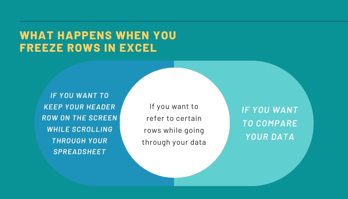

The feature is used to lock rows in some situations like.

• If you want to keep your row on the screen while scrolling through your.
• If you want to refer to certain topmost rows while going through your data.
• If you want to compare information.

This feature has many types of applications depending what you are using it for.

There are a few ways in which you can freeze your columns and rows. Go through the next section as the different methods have been comprehensibly described there.

Here’s a complete guide on how to Highlight Duplicates In Excel.

How to Freeze Rows and Columns in Excel

Excel lets you freeze one or more rows you want using the method but it can only freeze the rows starting from the top of the spreadsheet. This means that the tool cannot be used to hold up any specific row/rows in the middle of the sheet. The range will always start from the row at the top of your file.

Similarly, you can only freeze the leftmost column(s). Also, there is the option if you want to lock columns and rows together.

Note: If any row or column is out of view when you’re freezing them, they’ll continue to be hidden until you unfreeze them. So ensure the rows/columns you’re about to freeze are in sight.

The Freeze panes command has a few options, which can be used according to your preference and purpose of locking your rows/columns. There are a few ways you could do it and they are discussed clearly here.

Follow these steps to freeze rows and columns in Excel:

1. Freeze the Topmost Row

Spreadsheets usually have a header row on the top of all the data within the file that shows the label of a column’s data. While traversing through the content, there might be an issue with viewing the header row because as you move down, it moves away from the screen.

You won’t able to refer to the header if it isn’t on your screen.

So, you can lock the first row in place in Excel and prevent it from going off-screen when you scroll about on your file.

Here’s how to freeze the top row in Excel:

• Open your spreadsheet file.
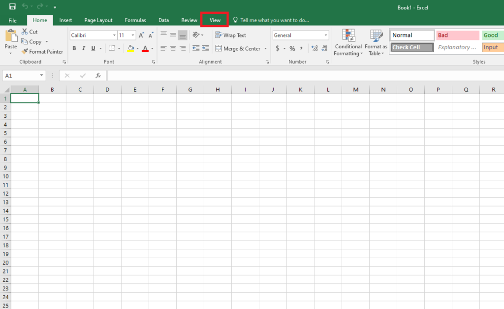
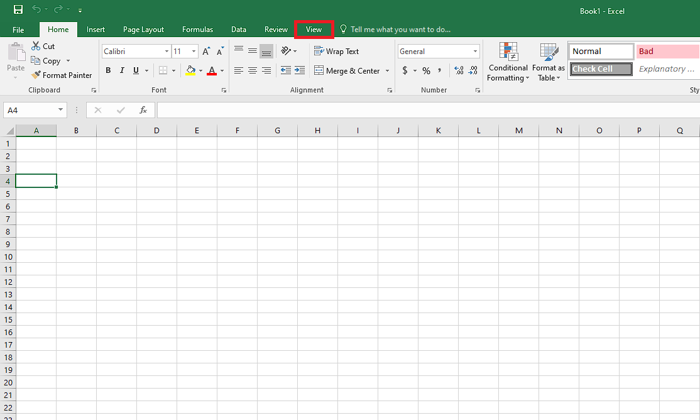
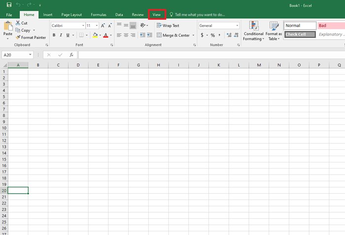
• Select the View tab after opening your file.
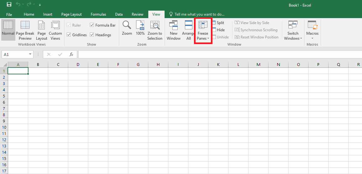
• Open the Freeze Panes tool menu.
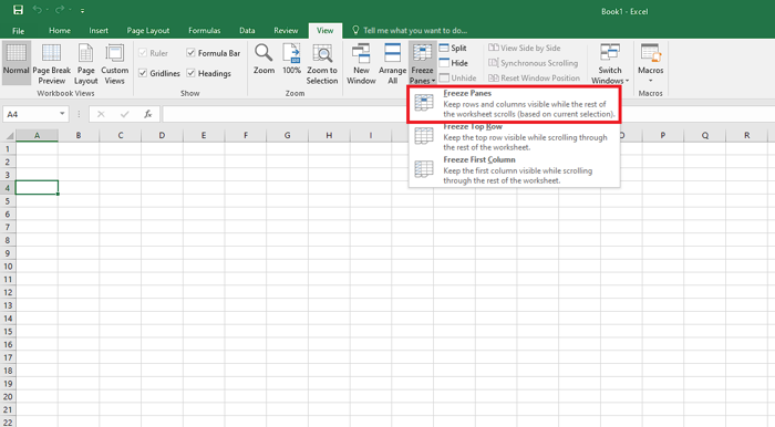
• Click on Freeze Top Row.

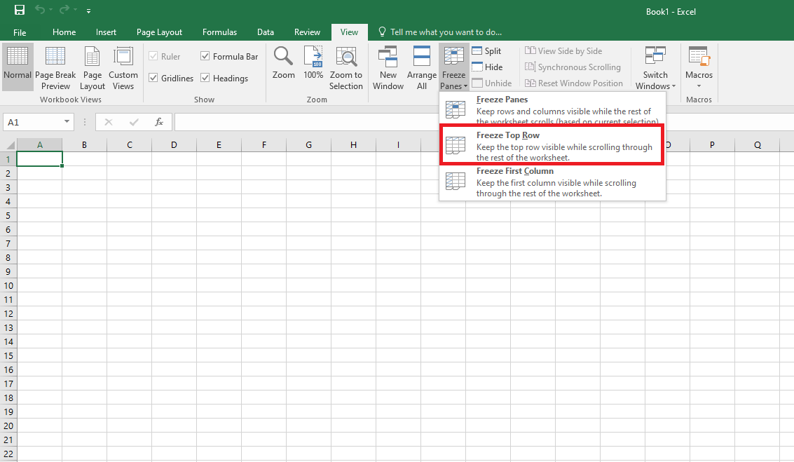
After you have followed this process, the top row of your file will now be held in place and you can see the content while continuing to view the bottom of the sheet.

Check our epic guide on how to Freeze Panes In Excel Easily.

2. Freeze Multiple Rows row

Excel provides the option to hold up any certain number of topmost rows you want at once. It means that those selected rows will be fixed on your screen. You can do this when you need to refer to some data or when it’s difficult to compare different sets of data contained within a workbook.

Go through these steps to freeze multiple rows in MS Excel:

• Open your worksheet file using Excel.
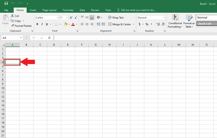
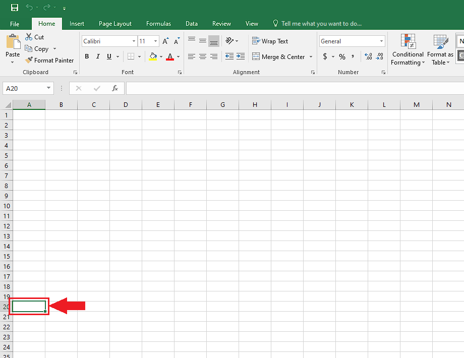
• Select the first cell right under the last row you want to freeze from top. For example, if you want to hold the first 3 rows, then you have to click on cell A4.
• Go to the View tab.
• Select the Freeze Panes menu.
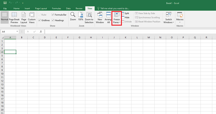
• Click on Freeze Panes.

Alternatively, you can select the row next to the last row you’d suspend. When you have gone through this method, the rows will now be grouped together, (indicated by a bold border under them) and be always visible on your screen. Scrolling won’t affect these rows as they have been held up

Also, check out our separate post on Microsoft Outlook not connecting to server.

3. Freeze the First Column

Spreadsheets often have the first column as a secondary header alongside the header row on the top. If you’re scrolling further right, there might be an issue with viewing the leftmost column as it moves away from the view.

Excel makes it easy to suspend the index column in view and prevent it from going off-screen.

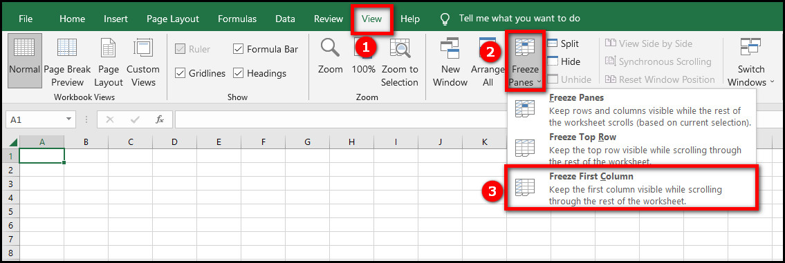
Here’s how to freeze the first column in Excel:

• Open your file in Excel.
• Select the View tab.
• Open the Freeze Panes tool menu.
• Click on the Freeze First Column option.

Now, the leftmost column of your file will be held in place and you can continue to view the frozen cells.

4. Freeze Many Columns

You can freeze any certain number of leftmost columns in place. Then those columns will always remain fixed on your screen.

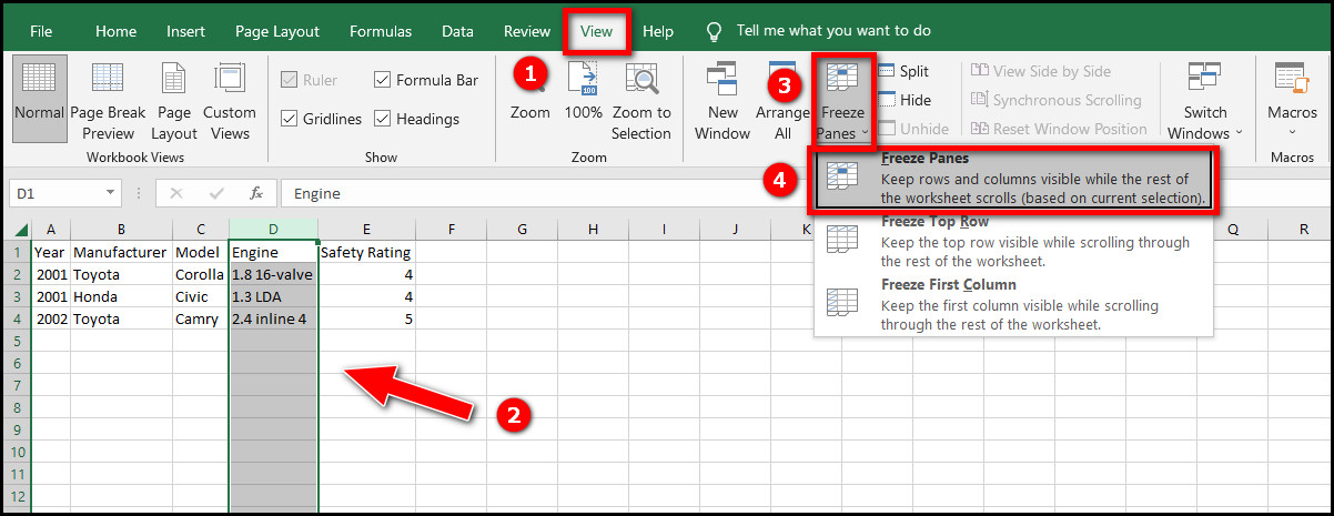
Go through these steps to freeze many columns in Excel:

• Open your spreadsheet file.
• Select the column right of the column you’d freeze. For example, if you want to hold the first 3 columns (A, B, C), then you have to select column D.
• Go to the View tab.
• Click the Freeze Panes option.
• Click on Freeze Panes.

The columns you wanted to freeze will now be grouped together, (indicated by a bold line next to them) and stay visible on your screen.

5. Freeze the Rows and Columns Together

Alongside freezing columns or rows separately, you can freeze them together. For example, you can suspend the topmost row and leftmost column at the same time.

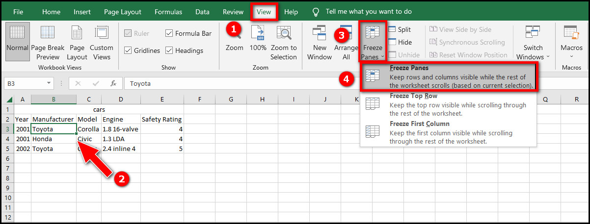
Here’s how to freeze multiple rows and columns in excel together:

• Open the worksheet file.
• Select the cell which is below the last row and right of the last column you’d freeze. For example, if you want to suspend the first two rows (1, 2) and column A, select cell B3.
• Go to the View tab.
• Click Freeze Panes > Freeze Panes.

That’s how you can freeze the columns and rows together in a single action.

5. Use Split tool to separate rows

Sometime it can be seen that with a huge amount of data, it is not possible to work as well by freezing. In these cases, you can use the split tool.

The Split tool separates your rows into halves that can be scrolled through independently.

It means that you can split your rows at any point within the sheet using this tool and the separated parts will now be independent of each other while being scrolled through. One can be kept stationary while another area is traversed and the two will never scroll at a time.

Take these steps to split rows in MS Excel:

• Run Excel and open your spreadsheet file.
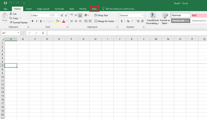
• Select any cell in the leftmost column.
  
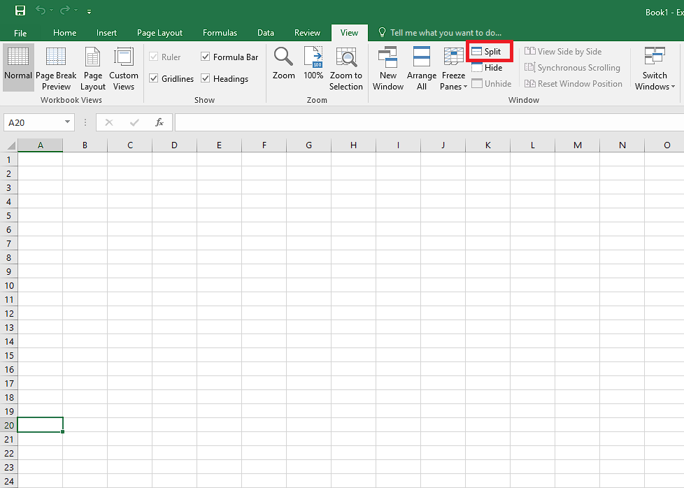
• Go to the View tab.
  
• Click on Split.

You will see that immediately your spreadsheet has been divided into two halves (indicated by a grey line) from the top of the cell that you had selected.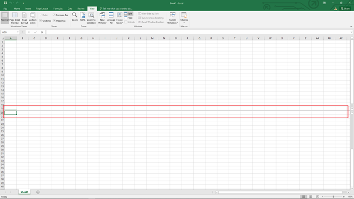

It will be as if you have two copies of your file on the same screen and you can traverse through them individually to compare two different data.

Here’s a complete guide on how to add someone to email thread Outlook.

How To Unfreeze Columns And Rows In Excel

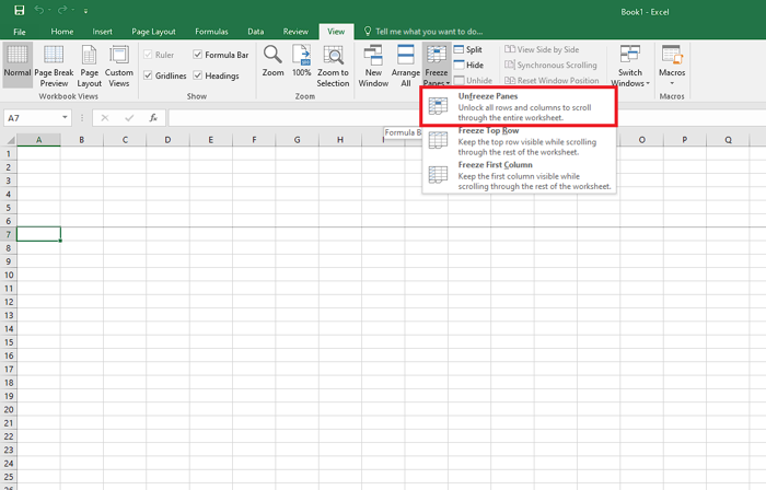
Suppose you make your columns and rows stationary in Excel, and you want to undo the action now. You can do it in a few clicks in Excel’s interface using Unfreeze Panes option.

To unfreeze your columns and rows, follow this process:

• Go to the View tab in Excel.
  
• Expand Freeze Panes menu for the options and select Unfreeze Panes.

Now, they will go back to what they were before.

Conclusion

Microsoft Excel has all sorts of tech that are necessary within a spreadsheet app and the option to make columns and rows static is one of the noteworthy features.

Writing and traversing through the rows of your spreadsheet file has never been more efficient than it is by suspending them. After appropriate selection, use the Freeze Panes in Excel to fix columns and rows in their place.

Learning how to freeze a column or row in MS Excel will help you make the most of your time. You can learn it quickly by following the methods in this guide.