Excel is not just a software service where you can only insert a few data tables and call it a day. There’s a myriad of applications when it comes to managing huge datasets in various manners, like finding the critical values for a normal or interval distribution.
Unfortunately, there’s no button that you can just press to find the desired value that you were looking for. You have to know the specific formula and how to use it properly in order to find the critical values in Excel, which is exactly what this article is all about.
So, without any delay, let’s get started.
What are Critical Values and Can They be Calculated in Excel?
Critical values are points on a distribution that define the boundary between non-significant and significant results in a hypothesis test. Depending on the significance level and the type of test, you may need to find one or two critical values for your data analysis.
In simple words, when you visualize a set of data as a graph, the critical values are the significant high or the significant low point/region of a distribution of values. These values can be about a country’s GDP, population growth, sales, etc.
Thankfully, since Excel is a widely used tool to analyze such large data sets, it has several built-in functions that can help us calculate critical values for different distributions, such as F, t, chi-square, and normal.
But, to find the subsequent critical values, each has a different formula and function that needs manual input in Excel. This brings us to our main topic.
How to Find Any Critical Values in Microsoft Excel
You can use the T.INV() function for the left-tail T distribution, ABS(T.INV()) for the right-tail, T.INV.2T() for the two-tail T distribution, and NORM.S.INV() function to calculate the Z critical value in Excel. However, you have to define the proper parameters to get the correct answer.
For example, if you use the T inverse function, you have to define the probability and degree of freedom to find the T critical value using the Excel formula.
So, how can you find those parameters? Well, let’s see with an example.
The probability or alpha parameter is usually one minus the confidence level converted to decimal. So, if our confidence level is 95%, then the probability is 1-.95=0.05. And for the degree of freedom, it’s always one less than the sample size.
Now, before we dive into the individual distributions, let’s see the universal way to calculate any mean value.
Here’s how to find critical values in MS Excel:
- Launch Excel and insert the set of data.
- Go to the Formulas tab and click on More Functions> Statistical.
- Select the distribution function for which you want to calculate the critical values. For demonstration, I’ve selected T.INV.2T.
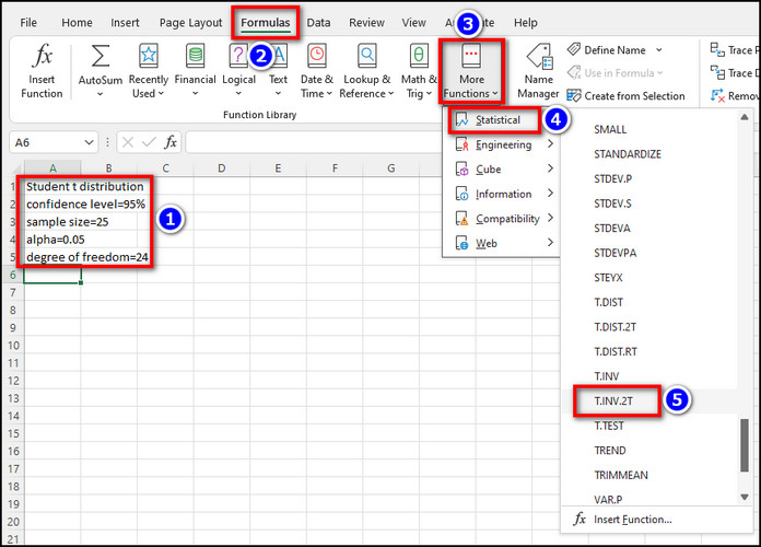
- Insert the probability and degree of freedom into their corresponding boxes and click on OK.
Done! You’ll get the results accordingly. Mind you, determine the defining parameters, like alpha value or degree of freedom, from the data set beforehand.
That was just one way to achieve the goal. But the story isn’t finished yet. You can input different pre-defined functions for different distributions directly into your spreadsheet and let Excel find the critical value for you.
Below, I have elaborated on the whole process and given step-by-step instructions for you to utilize the critical value formulas effectively.
How to Find T Critical Value in Excel
The interval estimate for a mean value, where the standard deviation for the data sample isn’t known, is usually calculated with the T inverse formula. This formula can change a bit depending on the type of T distribution value you want to find.
To be blunt, there are three types of T-sets for critical value: left-tail, right-tail, and two-tail. Each of these uses different functions to calculate the critical value accordingly. Such as:
Use the T.INV function for left tail T
Let’s say we have an alpha/probability of 0.05 and df(degree of freedom) of 24. The T.INV(probability, df) formula will give us the critical value for the left tail T-test.
So, for us, the input function will be =T.INV(0.05, 24). If we insert this function into your Excel spreadsheet and hit Enter, we’ll get -1.71088, which is our critical value in this scenario.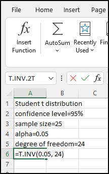
Use ABS(T.INV()) function for right tail T
To calculate the right-tail test, we need to combine the aforementioned T value Excel formula with the ABS function. After doing so, the formula stands as ABS(T.INV()).
So, let’s type =ABS(T.INV(0.05, 24)) into our spreadsheet and hit Enter. Voila! We get the right-tail critical value of 1.71088, which is the positive value of the left-tail test.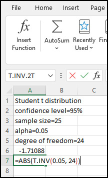
Use T.INV.2T function for two-tail T
Now, what about when we want to chop off both tails? For that, we’ll need to resort to the 2T function, which indicates two tails.
The final formula for that scenario stands as =T.INV.2T(0.05, 24). The result for the two-tail function comes as 2.06389.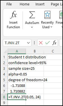
How to Find Z Critical Value for Normal Distribution in Excel
To calculate the critical value for normal distribution, you need to know the values for probability, mean, and standard deviation. After that, you can use the NORM.INV function for the non-standard curve.
Meanwhile, if you have a standard bell curve distribution, all you need is the probability and the NORM.S.INV function to find the Z critical value. Let’s see how it’s done.
Since there are three types of cases for a Z critical value(left tail, right tail, and two tail), the formula will see a slight change accordingly.
So, type =NORM.S.INV(probability) for left tail, =NORM.S.INV(1-probability) for right tail, and =NORM.S.INV(probability/2) for the two tail test. Then, press Enter on your keyboard to see the Z critical value in MS Excel.
On a side note, check out how to lock a cell in a formula in Excel.
How to Calculate Critical Value for Chi-Square Distribution in Excel
In case you’re working with chi-square distribution, use the CHISQ.INV(probability, df) or CHISQ.INV.RT(probability, df) function to find the corresponding critical values.
The first formula uses the left side of the graph as the probability of input, while the latter uses the right side of the graph.
To give a demonstration, let’s say the sample size you have is 38, and you have to find the critical value of standard deviation with a 95% confidence level estimate. Since you want to look at the area of each tail of the graph, the alpha would be 0.025 with a 37 degree of freedom.
So, the final formula reads as =CHISQ.INV(0.025, 37), which results in a 22.1056 critical value.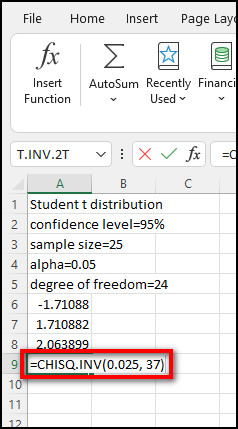
After all things said and done, you can measure the statistical significance of your hypothetical test by comparing each of these critical values.
To learn more about the mathematical functions, check out how to square a number in Excel.
Conclusion
The usefulness of this article in learning how to find critical values by using Excel is just as much as the usefulness of critical values for performing hypothetical tests for sales or other arrays of data.
Whether you’re a novice or well-versed in Excel, this write-up will surely be of assistance on the current matter.
Have a great day!