The true power of Excel lies not just in the data it holds but in the way you can manipulate it through the combination of formulas.
You can perform complex calculations by integrating various formulas within a single cell or across multiple cells. It allows you to create dynamic and interconnected spreadsheets where changes in the data set automatically update.
In this article, I’ll explain different ways to use two or more formulas in Excel, with easy-to-understand examples for each technique.
Let’s begin!
How to Use Multiple Formulas in One Cell in Microsoft Excel
You can leverage various functions and operators in Excel to perform complex calculations within a single cell. The ampersand operator (&) allows you to concatenate text or combine cell values. The CONCATENATE function also joins multiple cell values or text strings.
Additionally, the SUMIFS function helps you sum values based on multiple criteria. Nested functions enable you to create intricate logical conditions within a single formula.
By combining these functions creatively, you can create powerful formulas to perform diverse calculations.
Here are the methods to use multiple formulas in one cell in MS Excel:
1. Use the Ampersand (&) Operator
The ampersand symbol in Excel is used for concatenation, which means combining text or values. However, you need a different approach for joining two formulas, such as nesting the functions within each other.
Let’s say you have a column of numbers in cells A1 to A5. You want to calculate the sum and average of these numbers and combine the results into a single cell.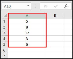
Enter the following formula in the cell where you want to display the result:
=”Sum: ” & SUM(A1:A5) & “, Average: ” & AVERAGE(A1:A5).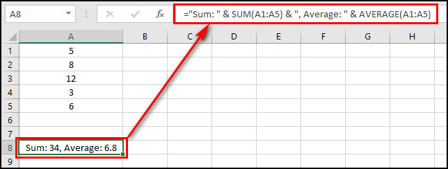
In this example, the SUM function calculates the sum of the numbers in cells A1 to A5, and the AVERAGE function calculates the average.
The results are then concatenated using the ampersand operator (&) and the desired text strings to create a combined result.
2. Utilize the CONCATENATE Function
CONCATENATE is a function in Excel that performs the same task as the ampersand (&) symbol. You can use this function to combine multiple calculations in a single formula.
Let’s say you have a set of numbers in cells A1 to A5, and you want to display both the average and sum in a single cell using CONCATENATE.
In another cell, you can use the following formula:
=CONCATENATE(“Average: “, AVERAGE(A1:A5), “, Sum: “, SUM(A1:A5)).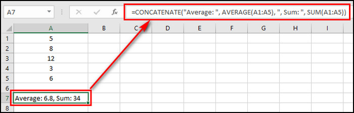
This formula combines the text ‘Average: ‘ with the result of the AVERAGE function for the range A1:A5, followed by ‘Sum: ‘ and the result of the SUM function for the same range.
3. Apply the SUMIFS Function
The SUMIFS function in Excel allows you to sum values based on different conditions. So, this formula calculates the total value only if a particular term is matched.
Let’s assume you have a dataset with sales data, and you want to find the total sales for a specific product in a particular region. In that case, use the SUMIFS formula.
Suppose you have the following data: 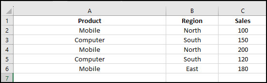 Now, to find the total sales for Mobile in the North region, enter the following SUMIFS function:
=SUMIFS(C2:C6, A2:A6, “Mobile”, B2:B6, “North”).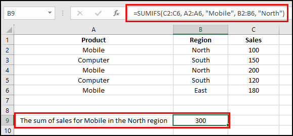
This formula sums the values in column C (Sales) where column A (Product) is equal to ‘Mobile,’ and column B (Region) is equal to ‘North.’
In this example, it would return the sum of sales for Mobile in the North region, which is 300.
You can also apply the SUMIFS function to combine formulas in a single cell by nesting them like the following technique:
=SUMIFS(C2:C6, A2:A6, “Mobile”, B2:B6, “North”) + SUMIFS(C2:C6, A2:A6, “Computer”, B2:B6, “South”).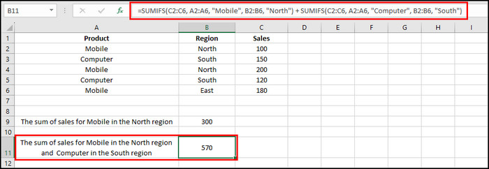
This formula calculates the sales for Mobile in the North region and adds it to the sales for Computer in the South region.
4. Use Nested Functions in a Formula
Nested functions involve using one function within another. It uses one function’s output as an argument for the other function. For example, you can apply the AND function inside the IF function to conditionally produce results.
Let’s say you have a dataset in Excel with two columns: Sales (column A) and Expenses (column B).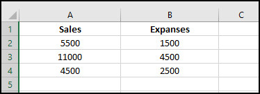
You want to calculate the profitability based on the following conditions:
- If sales are greater than $10000, and expenses are less than $5000, label it as ‘Highly Profitable.’
- If sales are greater than $5000, and expenses are less than $2000, label it as ‘Profitable.’
- If none of the above conditions are met, label it as ‘Not Profitable.’
You can use nested IF and AND functions to achieve this in a single cell.
Assuming your data starts from row 2, enter the following formula in the cell C2:
=IF(AND(A2>10000, B2<5000), “Highly Profitable”, IF(AND(A2>5000, B2<2000), “Profitable”, “Not Profitable”)).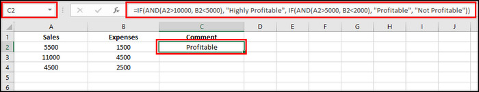
This formula checks the conditions individually and returns either Highly Profitable, Profitable, or Not Profitable in Comment (C column).
You can drag this formula down to apply it to other rows in the dataset. You might need to adjust the cell references based on your data.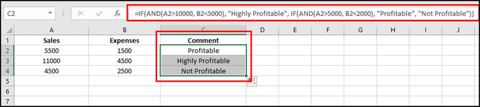
5. Utilize the CHOOSE Function
The CHOOSE function in Excel allows you to select a value from a list of choices based on a condition you’ve specified. You can combine it with other functions to choose among different formulas according to a condition.
Let’s assume you have a dataset in Excel with two columns: Score (column A) and Grade (column B).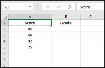
Now, if you want to assign grades based on the scores, use the CHOOSE function. Suppose you want to assign grades as follows:
- If the score is greater or equal to 90, the grade is A.
- If the score is between 80 and 89, the grade is B.
- If the score is between 70 and 79, the grade is C.
- If the score is less than 70, the grade is F.
Enter the following formula in cell B2 and drag it down for other cells in column B (Grade):
=CHOOSE(IF(A2>=90, 1, IF(A2>=80, 2, IF(A2>=70, 3, 4))), “A”, “B”, “C”, “F”).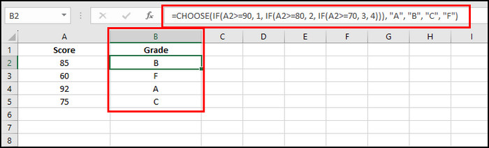
After entering this formula, the grades corresponding to the scores in column A should appear in column B. This example uses the nested IF functions within the CHOOSE function to evaluate the conditions and return the correct grades.
6. Apply Nested SUBSTITUTE Function
In Excel, the SUBSTITUTE function replaces a specified string with another string within a given text. The nested SUBSTITUTE function involves using SUBSTITUTE within SUBSTITUTE, creating a cascading effect of replacements.
The syntax for the substitute function is as follows:
SUBSTITUTE(text, old_text, new_text).
Where ‘text’ is the original string on your dataset, ‘old_text’ is the text you want to replace, and ‘new_text’ is the string that will replace the ‘old_text.’
Suppose you have a list of product codes in column A and want to clean up the codes by removing a specific prefix and suffix.
Here’s how you could use nested SUBSTITUTE functions to achieve this:
Let’s assume you have the following product codes: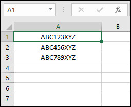
You want to remove the ABC prefix and XYZ suffix from the codes. For that, use the following formula in another column:
=SUBSTITUTE(SUBSTITUTE(A1, “ABC”, “”), “XYZ”, “”).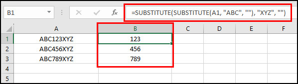
This formula uses two nested SUBSTITUTE functions. The inner SUBSTITUTE removes the ABC prefix from the original product code, and the outer SUBSTITUTE removes the XYZ suffix from the result of the inner SUBSTITUTE.
Things to Remember When Combining Multiple Functions into the Same Formula in Excel
When working with formulas, it is crucial to maintain consistency in data types to ensure accurate and meaningful results. Whether combining text or working with numeric values, you should always align the data types. Otherwise, the formula will generate errors in Excel.
For instance, confirm that both formulas produce text outputs when merging text. Similarly, when dealing with numerical data, verify that the combined values are numeric.
Mismatched data types can lead to errors and unexpected outcomes in your calculations.
Microsoft Excel is sensitive to the types of data it handles. So, combining incompatible types from different functions in a single formula will result in errors.
Additionally, parentheses are crucial when creating multiple formulas for the same space in Excel. By encapsulating specific segments of a formula within parentheses, you can ensure the formula is executed in the correct order.
Final Thoughts
With the combined power of different functions in Excel, data analysis and manipulation have just become much more straightforward. Seamlessly merging functions and formulas simplifies complex calculations and boosts productivity.
Comment below if you have further questions, and we’ll reply.